

When evaluating projects, comparing products, or scoring applicants, we often need to give more importance to certain variables or criteria than others. For fair calculation, we assign different weights to different variables.
Instead of manually working on each cell, automate the weight assigning process with Excel formulas. First, you need to enter the weights in a range and use the cell references in a formula with the SUMPRODUCT function.
➤ To assign weights and get the sum of the weighted values, enter the following formula in an empty cell:
=SUMPRODUCT(B2:D2, {0.5,0.3,0.2})
➤ Here, B2:D2 contains the variables and 0.5, 0.3, and 0.2 are the weights we want to assign to the columns of this range. Change the values as needed.
➤ Press Enter and drag the formula down to get the final output after assigning weights to your selected range and summing up the weighted results.
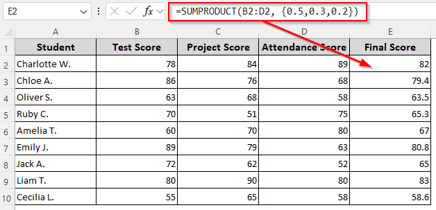
In this article, you’ll learn all the ways of assigning weights to variables using various functions like SUMPRODUCT, SUM, and VLOOKUP.
Using Simple Multiplication to Assign Weights and Sum
Our sample dataset has columns for Student names, Test Score, Project Score, Attendance Score, and Final Score. While assigning weights, make sure they are entered as percentages or their decimal equivalents (e.g., 50%, 30%, 20% or 0.5, 0.3, 0.2).
If you use percentages, the total of all weights must be 100% (e.g., 50% + 30% + 20% = 100%). When you use decimals instead, the total must be 1 (e.g., 0.5 + 0.3 + 0.2 = 1).
We’ll assign 0.5 to the Test Score column, 0.3 to the Project Score, and 0.2 to the Attendance Score. The summed weighted values will be in the Final Score column.
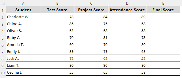
Here’s how to manually apply the weights to each column and get the summed final score:
➤ In the cell where you want the final summed value (E2), insert any of the following formulas:
Entering Weights Directly in Formula
If you don’t want to put the weights in a separate range and use them directly in the formula, enter:
=(B2*0.5) + (C2*0.3) + (D2*0.2)
➤ Here, B2, C2, and D2 are the first cells of the columns containing the variables and 0.5, 0.3, and 0.2 are the weights for each range. Replace the values according to your dataset. You can also use percentages instead of decimals.
➤ Press Enter and drag the formula down. This formula multiplies the weights of the variables in the column and sums up the multiplied numbers from all three columns.
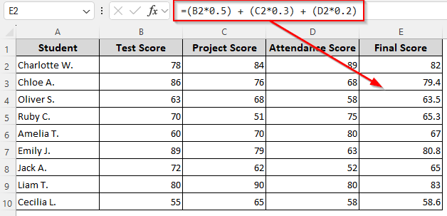
Entering Cell References in a Formula
Place the weights in cells B13, C13, and D13. In cell E2, enter:
=(B2*$B$13) + (C2*$C$13) + (D2*$D$13)
➤ Replace the cell references as needed.
➤ Click Enter and drag the formula down to get the final sum of weighted variables.
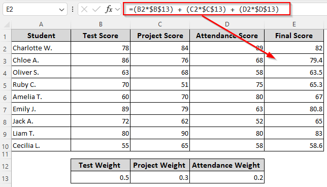
Manually Assigning Weights to Variables (Without Sum)
If you only want to assign weights to variables and get the multiplied results without summing up later, you can use a multiplication formula and enter the weighted values in a new range. Follow the steps given below:
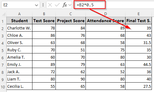
➤ We’ll put the weighted variables in Columns E, F, and G. So, in E2, we entered:
=B2*0.5
➤ Press Enter and drag the formula down to autofill the remaining cells.
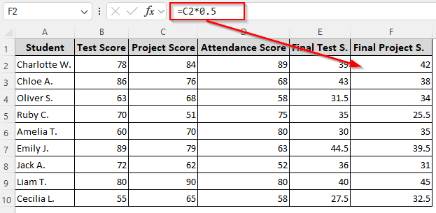
➤ Now, in F2, enter this formula, press Enter, and drag down.
=C2*0.5
➤ Finally, in G2, enter this formula, press Enter, and drag down.
=D2*0.5
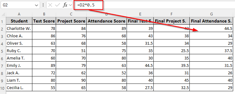
➤ Repeat the steps for more columns if you have any. Change the cell reference to the first cell of the column.
Assigning Weights and Summing Up with the SUMPRODUCT Function
In this method, we’ll use a formula that takes your data row (scores) and multiplies each number by its importance (weight), then adds them all up. Here’s how:
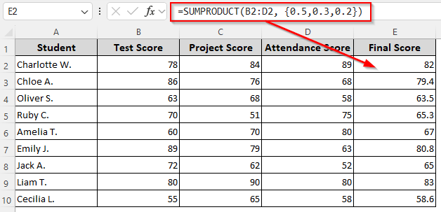
➤ In an empty cell where you want to sum of weighted values, enter this formula:
=SUMPRODUCT(B2:D2, {0.5,0.3,0.2})
➤ In the range B2:D2, we have the first cells of each column containing the variables. For Columns B, C, and D, we’re assigning the weights 0.5, 0.3, and 0.2, respectively. Change the values as needed. Use direct percentages or cell references if you prefer.
➤ Press Enter and drag the formula down.
Handling Weights That Are Integers and Don’t Sum to 100 (Not Decimals or Percentages)
If your weights are integers (e.g., 50, 40, 20) instead of decimals or percentages and they don’t sum to 100, we need to alter the SUMPRODUCT formula to make sure the final score is on the same scale. Below are the details:
➤ Select the cell where you want the final summed value (E2), enter any of the following formulas:
Entering Weights Directly in the Formula
To use the weights directly in the formula, enter:
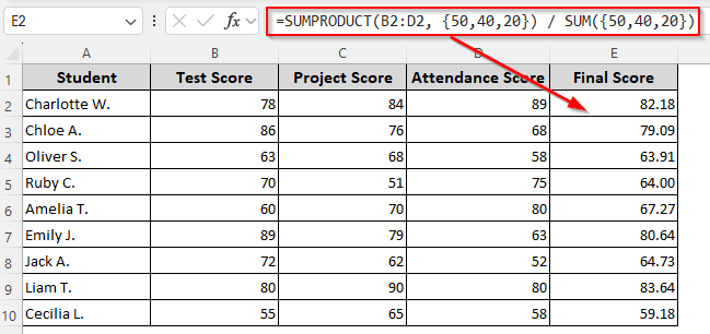
=SUMPRODUCT(B2:D2, {50,40,20}) / SUM({50,40,20})
➤ Here, B2:D2 contains the variables and 50, 40, and 20 are the weights. Change the values to match your dataset.
➤ Click Enter and drag the formula down.
Entering Cell References in a Formula
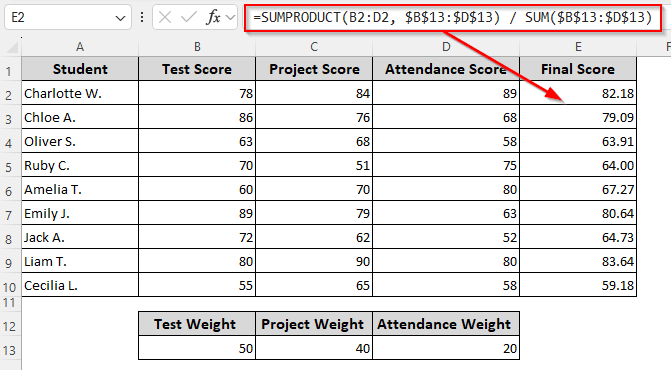
Insert the weights in cells B13, C13, and D13. In an empty cell, enter:
=SUMPRODUCT(B2:D2, $B$13:$D$13) / SUM($B$13:$D$13)
➤ Replace the cell references as required.
➤ Press Enter and drag the formula down for the final adjusted weighted sum.
Dynamically Assign Weights Based on Text Variables and Sum
Instead of manually assigning the weights to specific variables, we can automate the process with VLOOKUP. First, we’ll create a weight table with the list of variables and weights.
After that, we’ll use a formula that looks for the variable name in the sheet, assigns a specified weight for the matching values, and calculates the sum of the weighted range. Let’s get to the steps:
➤ To create a weight table, enter the variables and weights in two adjacent columns. We put the variable names in the range B13:B15 and the weights for each range in C13:C15.
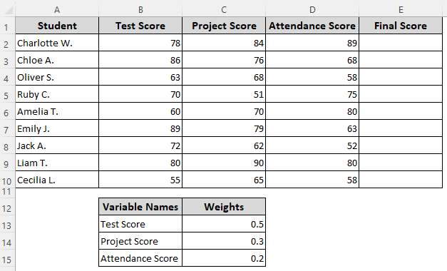
➤ In the cell where you want the summed values (E2), enter the following formula:
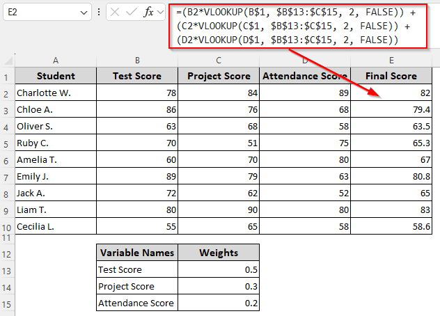
=(B2*VLOOKUP(B$1, $B$13:$C$15, 2, FALSE)) + (C2*VLOOKUP(C$1, $B$13:$C$15, 2, FALSE)) + (D2*VLOOKUP(D$1, $B$13:$C$15, 2, FALSE))
➤ Here, cells B1, C1, and D1 contain the variable names, and B2, C2, and D2 contain the first values on which we’ll assign weights. $B$13:$C$15 is the weight table range. Replace these references to match your source data. You can add more columns following the same pattern.
➤ Click Enter and drag the formula down to get the summed weighted values for all the rows.
Note:
If you don’t want to sum the weighted values, you need to insert a formula for each column containing the variables. For example, this is the formula for Column B:
=B2*VLOOKUP(B$1, $B$13:$C$15, 2, FALSE)
Downloadable Resources
Get our practice workbook or necessary files that we have worked with to prepare this article.
Assigning Weights to Variables.xlsx
Frequently Asked Questions
How to apply the weighted average formula in Excel?
To calculate a weighted average in Excel, multiply each value by its assigned weight, add the results, and divide by the total of all weights. Select the cell for the result and enter this formula:
=SUMPRODUCT(B2:D2, {0.5,0.3,0.2}) / SUM({0.5,0.3,0.2})
Adjust the ranges and weights. Press Enter and drag the formula down if needed.
How to create a weighted ranking?
For weighted ranking (rank items based on weighted scores), first, calculate each item’s weighted score using this formula (in E2):
=SUMPRODUCT(B2:D2, {0.5,0.3,0.2})
Replace the range and weights as needed. Press Enter and drag the formula down for all rows. To rank the summed weighted values, use the RANK.EQ or RANK function:
=RANK.EQ(E2, $E$2:$E$10, 0)
Here, 0 is for descending order (higher scores get higher ranks). You can use 1 for ascending order. Change the range as required. Press Enter and drag the formula down.
How to make charts with weighted values in Excel?
To create a visual chart, calculate the weighted scores using your chosen formula. Select the names (e.g., Students) and their weighted scores. Go to the Insert tab >> Charts >> choose a chart type. Use a Column Chart for comparisons, a Line Chart for performance trends, and a Radar Chart is great for multi-criteria comparison.
Concluding Words
Choose a method depending on whether you want to get only the weighted values or add them to get an average score. If you want to update the weights later, insert the weights in your sheet and use cell references in the formula. This way, you can update values without altering the formulas.