INDEX-MATCH with Multiple Criteria Across Rows and Columns

A simple INDEX-MATCH formula handles single criteria, but when you need to match both rows and columns with multiple criteria, you need more advanced formulas. By default, MATCH finds the position of your lookup value and INDEX uses that position to return the corresponding value.

If your lookup values are across multiple columns or rows, you must combine more functions like SMALL, ROW, IF, etc., to get your desired outcome.

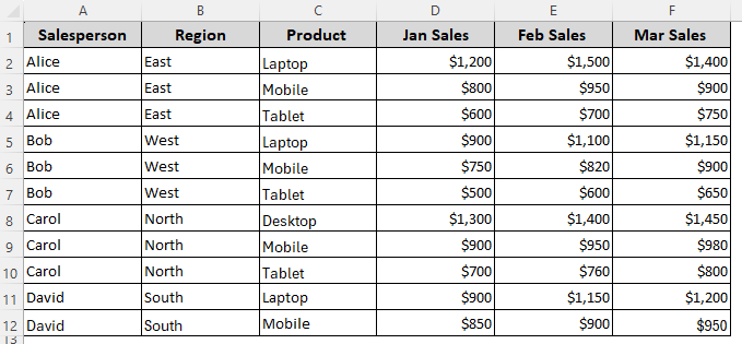
In our sample dataset, we have a few salesperson’s names in Column A, regions in Column B, product names in Column C, and monthly sales for January, February, and March are in Columns D, E, and F. Our goal is to find a match based on multiple criteria where the criteria are in the same or different rows/columns.

Depending on the outcome you want, choose any of the following ways:

Two Criteria in the Same Row

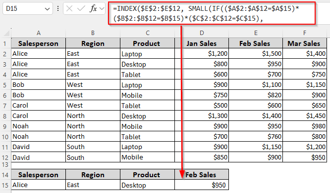
Use this formula to match the row with our specified Salesperson (from A15) and Product (from B15) and return the corresponding Feb Sales figure  from Column E.

➤ If you want to return the sales value where Salesperson=Alice and Product=Tablet, enter the two criteria in A15 and B15. Now, insert this formula in C15:

➤ To match your source data, replace the lookup ranges $A$2:$A$12 and $C$2:$C$12, first cell of the first lookup range $A$2, return range $E$2:$E$12, and reference cells $A$15 and $B$15.
➤ In Excel 365/2021, press  Enter  . For older versions, click  Ctrl  +  Shift  +  Enter  .
➤ If there are multiple matches, drag the formula down until it returns an error.

Two Criteria in the Same Column

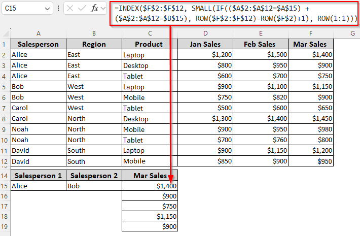
This formula finds Alice (from A15) and Bob (from B15) in Column A and then returns the corresponding Mar Sales from Column F.

➤ To find the sales values for Alice and Bob in March, enter the values A15 and B15. Insert this formula in C15:

➤ Change the values and ranges as needed.
➤ Press  Enter  or  Ctrl  +  Shift  +  Enter  depending on your Excel version.
➤ Drag the formula down to get all the prices.

In this case, our lookup is based on 3 criteria in the same row/column. Based on the result you want, follow any of the given methods:

Three Criteria in the Same Row

Here, we’ll find the Feb Sales for a specific Product, sold by a specific Salesperson, for a specific Region.

➤ Enter Alice in A15, East in B15, and product name Desktop in C15. Use this formula to get the Feb Sales matching all three criteria:

➤ To match your source data, change the lookup ranges $A$2:$A$12, $C$2:$C$12, and $C$2:$C$12, first cell of the first lookup range $A$2, reference cells $A$15, $B$15, and $C$15, and the return range $E$2:$E$12.
➤ Click  Enter  or  Ctrl  +  Shift  +  Enter  based on your Excel version.
➤ Drag the formula down to get all the matches.

Three Criteria in the Same Column

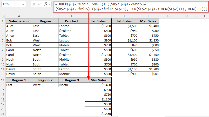
Use this method to find the Mar Sales (Column F)figures based on the specified regions from Column A.

➤ To find the sales numbers for the East, West and North regions in March, enter the three values in A15, B15, and C15. Insert this formula in D15:

➤ Replace the values and ranges according to your dataset.
➤ Press  Enter  or  Ctrl  +  Shift  +  Enter  , depending on your Excel version, and drag the formula down.

When your criteria lie in a single row and 2 different columns, use this method to get your desired outcome based on those 3 criteria.

If A15 contains the Salesperson’s name, B15 contains the Region, and C15 contains the Product, this formula returns the Jan Sales using the row criteria (Salesperson) and column criteria (Region and Product). Below are the details:

➤ Insert Bob in A15, West in B15, and product name Mobile in C15. To get the Jan Sales where the row criteria match any of the column criteria, use this formula:

➤ Replace the lookup ranges $A$2:$A$12, $B$2:$B$12, $C$2:$C$12, first cell of the lookup range $A$2, reference cells $A$15, $B$15, and $C$15, and the return range $D$2:$D$12 as required.
➤ Depending on your Excel version, press  Enter  or  Ctrl  +  Shift  +  Enter  .
➤ Drag the formula down to get all the matches.

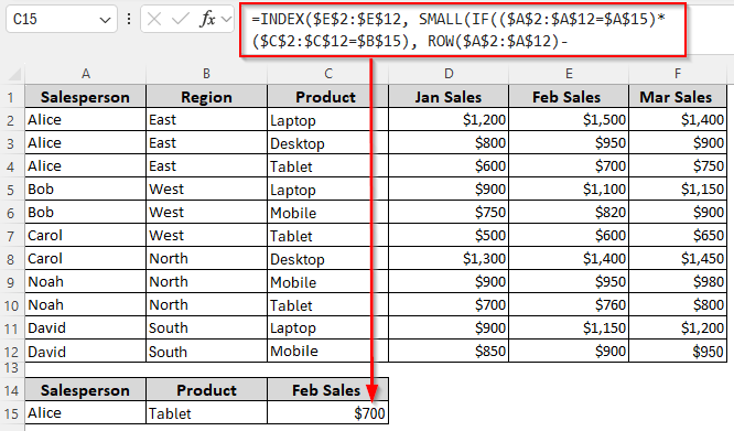
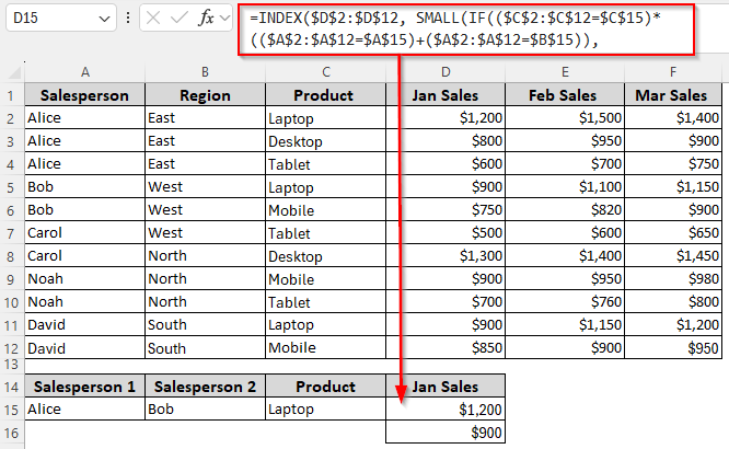
For this method, we’ll use 2 criteria from different rows of the same column and one from a different column. When A15 and B15 contain the Salesperson’s names from Column A and C15 contains the Product from Column C, this formula returns the Jan Sales using the row criteria (Salesperson) and column criteria (Product). Here are the steps:

➤ Enter Alice in A15, Bob in B15, and Laptop in C15. Insert this formula in D15 to get the Jan Sales figures where the column criterion matches any of the row criteria:

➤ To match your source data, adjust the lookup ranges $A$2:$A$12 and $C$2:$C$12, first cell of the lookup range $A$2, reference cells $A$15, $B$15, and $C$15, and the return range $D$2:$D$12.
➤ Click  Enter  or  Ctrl  +  Shift  +  Enter  based on your Excel version.
➤ Drag the formula down for all matching results.

Here, we’ll use INDEX-MATCH to find a product matching the numeric criteria we set for all 3 months (Jan, Feb, and Mar). Choose any of the methods given below based on the outcome you want:

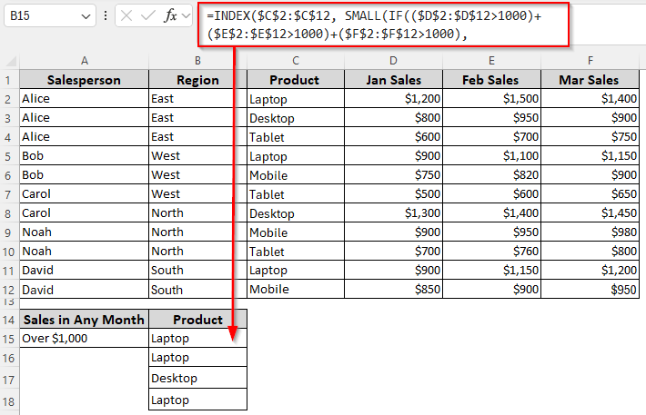
Find Values When At Least One Column Matches the Criteria

➤ If you want to find the Product(s) generating over $1,000 in any month, use the following formula:

➤ Replace the lookup ranges $D$2:$D$12, $E$2:$E$12, $F$2:$F$12, return range $C$2:$C$12, and first cell of the return range $C$2:$C$12 according to your dataset.
➤ Press  Enter  or  Ctrl  +  Shift  +  Enter  depending on your Excel version.
➤ Drag the formula down for all matching values.

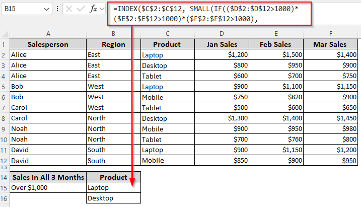
Find Values When All Columns Match the Criteria

To find the Product(s) generating over $1,000 in all 3 months, enter this formula:

➤ Replace the ranges as needed to adjust the formula for your source data.
➤ Click  Enter  or  Ctrl  +  Shift  +  Enter  based on your Excel version.
➤ Drag the formula down for multiple matches.

Frequently Asked Questions

What is the alternative to INDEX-MATCH for multiple criteria?

The most common alternative to INDEX-MATCH is the FILTER function (Excel 365/2021). If A15=Bob (Column A), B15=Carol (Column A), and C15=Laptop (Column C), you can use this formula with FILTER to return the matching Jan Sales (Column D):

=FILTER($D$2:$D$12, ($C$2:$C$12=$C$15)*(($A$2:$A$12=$A$15)+($A$2:$A$12=$B$15)))

This formula directly spills all values where Product=Laptop and Salesperson=Bob or Carol. Change the ranges as needed and press Enter.

How to handle errors with an INDEX-MATCH formula?

You can wrap your INDEX-MATCH formula with IFERROR so that blank cells (or custom messages) appear instead of errors. To return Jan Sales from Column D where Laptop (Column C) matches to Bob or Carol (Column A), use this formula to handle errors:

=IFERROR(INDEX($D$2:$D$12, SMALL(IF(($C$2:$C$12=$C$15)*(($A$2:$A$12=$A$15)+($A$2:$A$12=$B$15)), ROW($C$2:$C$12)-ROW($C$2)+1), ROW(1:1))), "")

If no match is found, the formula will return a blank (“”). Adjust the references to fit your dataset and press Enter or  Ctrl  +  Shift  +  Enter  depending on your Excel version.

Does INDEX-MATCH return results horizontally?

By default, INDEX-MATCH works vertically, but you can adapt it to return horizontal results by flipping the logic. For example, if your dataset has months (Jan, Feb, Mar) across Row 1 (D1:F1) and you want the Jan Sales for a specific Salesperson and Product (criteria in A15, B15, and C15), you can adjust the formula like this to return results horizontally:

=INDEX($D$2:$F$12, MATCH($A$15&$B$15, $A$2:$A$12&$C$2:$C$12, 0), MATCH($C$15, $D$1:$F$1, 0))

Replace the values and press  Enter  or  Ctrl  +  Shift  +  Enter  based on your Excel version.

Concluding Words

Choose the correct method depending on whether you’re going for the same row lookup, same column lookup, or get values from multiple columns for one product.

All our formulas can return multiple matches, so you need to drag them down until you get the #N/A error. To replace the error with a blank, wrap your formula with the IFERROR function.