When working with large datasets in Excel, we often need to look up values based on multiple criteria. The INDEX and MATCH functions are powerful built-in tools that allow us to perform this task efficiently in Excel.
Follow the steps below to look up a value in the dataset with three different criteria using the INDEX and MATCH functions:
➤ In your dataset, head to the cell where you want to display the lookup value and paste the following formula:
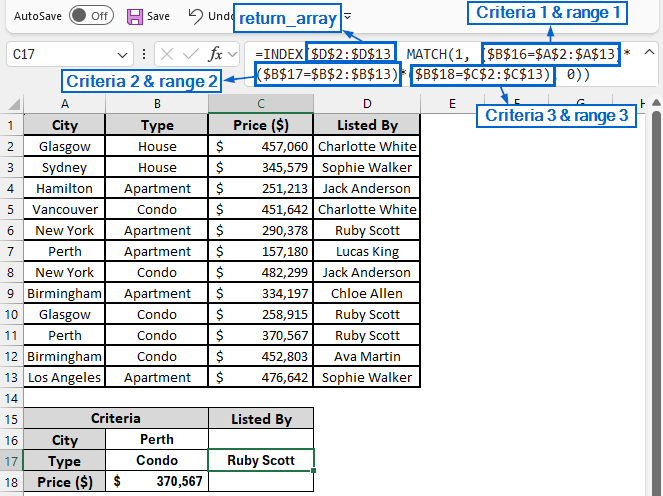
=INDEX(return_array, MATCH(1, (criteria1=range1)*(criteria2=range2)*(criteria3=range3), 0))
➤ Replace return_array with the column or range from which you want to extract the result.
➤ Replace criteria1 with the cell reference containing the first lookup value.
➤ Replace range1 with the column or range that should be matched against the first criteria.
➤ Replace criteria2 with the cell reference containing the second lookup value.
➤ Replace range2 with the column or range that corresponds to the second criteria.
➤ Replace criteria3 with the cell reference pointing to the third lookup value.
➤ Replace range3 with the column or range where the third criteria will be matched.
In this article, we will explore four effective methods of using the INDEX and MATCH functions to look up values based on three criteria in Excel.
Use Array Formula with INDEX and MATCH for Three-Criteria Lookup
In the sample dataset, we have a worksheet called “Real Estate Details” containing information about City, Type, Price and name of the person who listed each property.
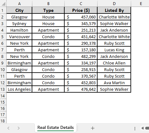
Using an array formula with INDEX and MATCH, we will find who listed the property based on the City, Type, and Price criteria. The updated dataset will be stored in a separate worksheet called “INDEX+MATCH Array Formula”.
An array formula in Excel is a special type of formula that can perform multiple calculations on one or more sets of values and return either a single or multiple results. When combined with the INDEX and MATCH functions, it allows users to look up values based on multiple criteria.
Steps:
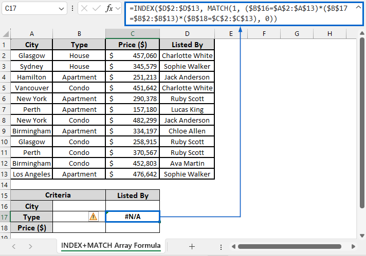
➤ Open the INDEX+MATCH Array Formula worksheet and in cell C17 paste the following formula:
=INDEX($D$2:$D$13, MATCH(1, ($B$16=$A$2:$A$13)*($B$17=$B$2:$B$13)*($B$18=$C$2:$C$13), 0))
➧ INDEX($D$2:$D$13, … ) part extracts a value from column D (D2:D13), which is the return column.
➧ MATCH(1, … ,0) finds the row number where all specified conditions are met. “1” represents the point where all logical tests are TRUE, and “0” ensures an exact match.
➧ ($B$16=$A$2:$A$13) part compares the first lookup value in B16 against all rows in column A.
➧ ($B$17=$B$2:$B$13) checks the second lookup value in B17 against all rows in column B.
➧ ($B$18=$C$2:$C$13) compares the third lookup value in B18 against all rows in column C.
➧ (...) * (...) * (...) multiplies the three logical arrays together.
➧ MATCH(1, … ,0) determines the position of the row where all criteria are met.
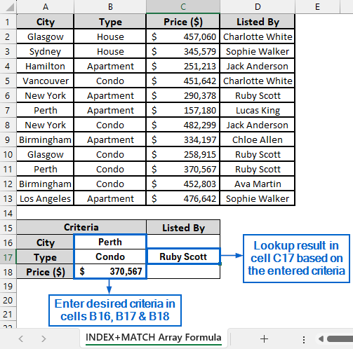
➤ Next, enter the desired criteria in cells B16, B17, and B18 then press Enter.
➤ Search result based on the entered criteria should now be displayed in cell C17.
INDEX MATCH Without Array Formula
Unlike the previous method, this approach uses a regular INDEX–MATCH formula rather than an array formula to evaluate multiple criteria simultaneously.
Using the same dataset, we will return a value in cell C17 based on three different criteria, this time without applying an array formula. The modified dataset will be stored in a separate “INDEX+MATCH No Array Formula” worksheet.
Steps:
➤ Open the INDEX+MATCH No Array Formula worksheet and in cell C17 type the following formula:
=INDEX($D$2:$D$13, MATCH(1, INDEX(($B$16=$A$2:$A$13)*($B$17=$B$2:$B$13)*($B$18=$C$2:$C$13),0,1), 0))
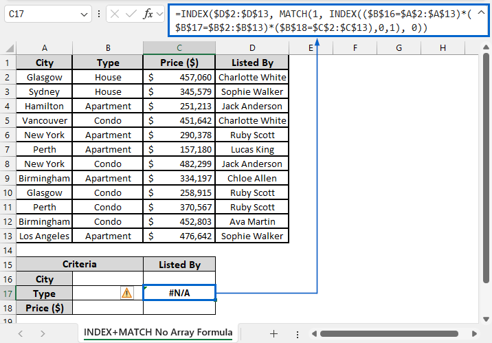
➧ INDEX(($B$16=$A$2:$A$13)*($B$17=$B$2:$B$13)*($B$18=$C$2:$C$13),0,1) part converts the array of multiplied TRUE/FALSE values into a single-column array so that MATCH can process it correctly.
➧ MATCH(1, ..., 0) finds the position where all three criteria are met.
➧ INDEX($D$2:$D$13, …) retrieves the corresponding value from column D based on the position found.
Everything else works the same as in the previous method.
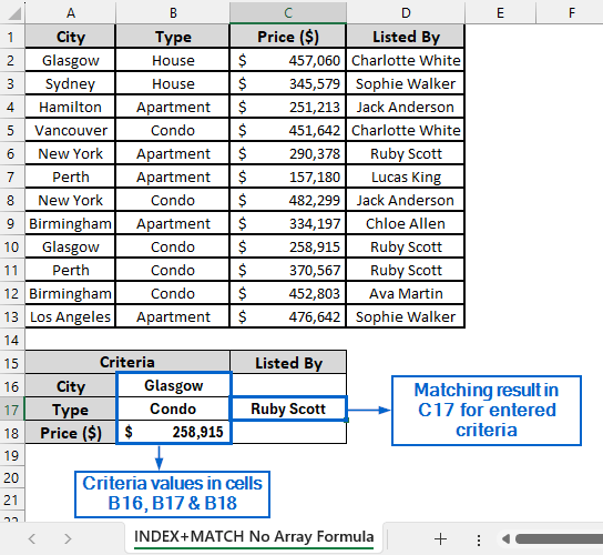
➤ Now, input your criteria values into cells B16, B17, and B18.
➤ The matching result for those entered criteria will automatically appear in cell C17.
Use IFERROR and INDEX-MATCH for Lookup with Error Handling
IFERROR is a useful Excel function that helps users manage and suppress errors in formulas. Unlike other methods, by combining IFERROR with INDEX and MATCH, we can perform multi-criteria lookups while displaying a custom message or value when no match is found.
Working again with he same dataset, we will now apply IFERROR with INDEX and MATCH functions to display the result for three criteria search in cell C17. The updated dataset will be displayed in a separate worksheet called “INDEX+MATCH with IFERROR”.
Steps:
➤ Head to INDEX+MATCH with IFERROR worksheet and in cell C17 put the following formula:
=IFERROR(INDEX($D$2:$D$13, MATCH(1, INDEX(($B$16=$A$2:$A$13)*($B$17=$B$2:$B$13)*($B$18=$C$2:$C$13),0,1), 0)), "Not Available")
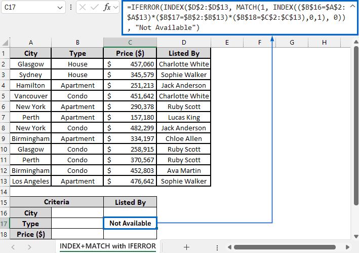
➧ IFERROR( … , "Not Available") part displays a message “Not Available” if the formula results in an error.
Everything else in the formula works the same as in the previous INDEX-MATCH method.
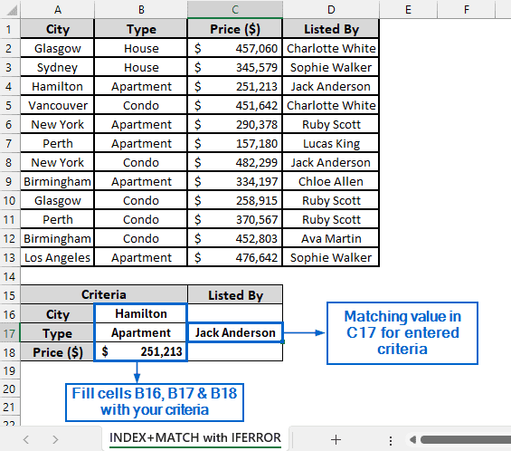
➤ Fill cells B16, B17, and B18 with the criteria you want.
➤ The matching value for entered inputs will appear in cell C17.
Combine TEXTJOIN with INDEX and MATCH for Multi-Criteria Search
TEXTJOIN is another useful tool in Excel that allows users to combine text from multiple cells into a single string, with a specified delimiter. By combining this with INDEX and MATCH functions, we can create a search box that returns a value based on multiple criteria.
Working again with the same dataset, we will now use TEXTJOIN with INDEX and MATCH functions to display results based on three criteria in cell C17. We will display the modified dataset in a separate “INDEX+MATCH with TEXTJOIN” worksheet.
➤ Open the INDEX+MATCH with TEXTJOIN worksheet and in cell C17 enter the following formula:
=INDEX($D$2:$D$13, MATCH(TEXTJOIN("|",,B16,B17,B18), $A$2:$A$13&"|"&$B$2:$B$13&"|"&$C$2:$C$13, 0))
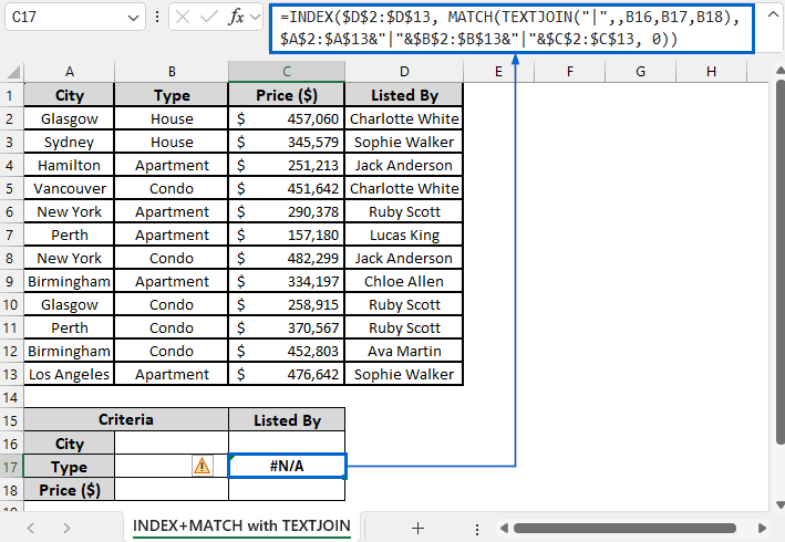
➧ TEXTJOIN("|",,B16,B17,B18) combines the three lookup values in B16, B17, and B18 into a single text string separated by “|” delimiter.
➧ ($A$2:$A$13&"|"&$B$2:$B$13&"|"&$C$2:$C$13) concatenates the three columns row by row into the same delimiter, creating a single array of combined keys.
➧ MATCH( ..., 0) ensures an exact match.
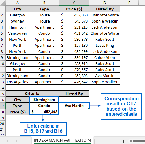
➤ Next, enter the desired criteria into cells B16, B17, and B18.
➤ The corresponding result based on these criteria will now be displayed in cell C17.
Frequently Asked Questions
Can I Use INDEX MATCH with More than 3 Criteria in Excel?
Yes, you can use INDEX and MATCH with more than three criteria in Excel. By multiplying additional logical conditions inside the MATCH function, you can evaluate as many criteria as needed.
What Happens If the Criteria Values are Case-Sensitive?
By default, INDEX and MATCH formulas in Excel are not case-sensitive. This means that “Apple” and “apple” will be treated as the same when performing lookups.
Which Method is More Suitable For Working With Large Datasets?
If you need to return a value based on three criteria from a large dataset, the INDEX and MATCH method without an array formula would be the most suitable. By retrieving only the required value without processing entire arrays or concatenated strings, it ensures faster and more efficient performance.
Concluding Words
Knowing how to INDEX-MATCH with three criteria in Excel is essential for performing multi-condition lookups and ensuring accurate results in complex datasets.
In this article, we have discussed four effective methods for using INDEX and MATCH in Excel with three criteria, including using an array formula, a non-array formula, and combining IFERROR and TEXTJOIN functions. Feel free to try out each method and select one that best aligns with your needs.