
When we work with business or academic data, using a simple average doesn’t always give an accurate result. Because, in most cases, some values carry more importance than others in this type of data. Thus, we need to use the weighted average.
For example, suppose you have sales data from different products, where some products contribute more to total revenue than others. So, simply averaging sales would ignore their true impact. Instead, using a weighted average will ensure that products with higher contribution percentages influence the final result more, and you can see the real scenario.
In this article, we will learn different methods to calculate the weighted average with percentages using the SUM and SUMPRODUCT functions in Excel.
➤ First, select cell A8 and write down a suitable name.
➤ Then, click on cell B8 and insert the following formula:
=SUM(B2*C2, B3*C3, B4*C4, B5*C5) / SUM(C2:C5)
➤ Finally, press Enter, and it will return the weighted average value.

What Is Weighted Average?
The weighted average is also a type of average. The only difference is that, in our ordinary average, every number has the same importance. However, in a weighted average, some numbers or points carry more importance, such as in an exam, where different courses have varying weights or credits.
Usually, while doing manual calculations for such cases, we multiply the grade of a particular course by the assigned weight or credit and then divide the sum of all the courses by the total weights.
Suppose a student has three courses where he got 80 in course A, 70 in course B, and 90 in course C. Course A, B, and C have assigned weights 2, 3, and 4, respectively. So, to calculate the weighted sum, first we will multiply each grade by its respective weight and sum all three numbers. That is, (80 × 2) + (75 × 3) + (90 × 4) = 160 + 225 + 360 = 745. Then, we divide 745 by the total credits: 2 + 3 + 4 = 9. So, the weighted average grade is 745 ÷ 9 = 82.78.
Calculate Weighted Average Using the SUM Function in Excel With Percentages
The SUM function helps us to add numbers in Excel. To calculate the weighted average, first, we will multiply each value by its percentage. Then, we will use the SUM function to add all those results together.
We will use the dataset below to explain the method of using the SUM function to calculate the weighted average in Excel with percentages.
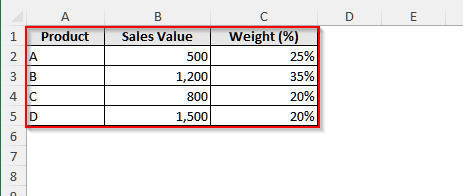
This is a sales dataset for a few products that have importance or weights.
Steps:
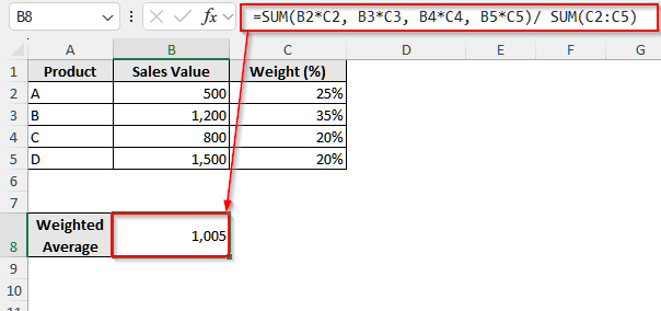
➤ First, click on cell A8 and write Weighted Average.
➤ Then, select cell B8 and insert the following formula:
=SUM(B2*C2, B3*C3, B4*C4, B5*C5) / SUM(C2:C5)
➤ Finally, press Enter, and it will return the weighted average value.
➤ Now, to calculate the normal average, select cell A9 and write Normal Average.
➤ Then, click on cell B9 and insert the following formula:
=AVERAGE(B2:B5)
➤ After that, press Enter, and you will see the normal average for the selected values.
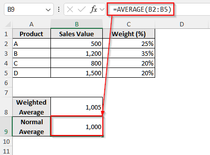
From the calculations, it is evident that the weighted average differs from the unweighted average. That is, in the case of weighted data, if we use the normal average value for evaluation, it will lead to inaccurate results, as it ignores the different importance of each value.
Using SUMPRODUCT Function to Calculate Weighted Average with Percentages
The SUMPRODUCT function multiplies each value by its percentage automatically and adds all the multiplied values. It is a great alternative to the SUM function. While the SUM function breaks down each step of calculating the weighted average and helps beginners to learn about the weighted average, it is not suitable for larger datasets. In such a case, we use the SUMPRODUCT function as it automatically does the calculations.
Steps:
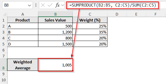
➤ First, select cell A8 and write a name for your later calculation.
➤ Then, click on scell B8 and insert the following formula:
=SUMPRODUCT(B2:B5, C2:C5)/ SUM (C2:C5)
➤ At last, press Enter, and the formula will return the weighted average value.
➥ Here, the function SUMPRODUCT is our starting part. This function tells Excel to do the latter calculation.
➥ The first range inside the parentheses, B2:B5, is the second part. In our data, this range represents the sales value. Remember, you need to replace this range with your value range.
➥ Then the second range, C2:C5, represents the weights. Inside the SUMPRODUCT function, Excel handles this expression, (B2:B5, C2:C5) as B2 × C2, B3 × C3, B4 × C4, and B5 × C5. That is, it automatically multiplies each cell in the first range by the corresponding cell in the second range.
➥ And the final part is SUM (C2:C5). We divide the whole SUMPRODUCT argument by this SUM (C2:C5) to get the weighted average. Remember, you must use the same range of weights inside this SUM function that you have used as the second range inside the SUMPRODUCT function. That is, in our case, it is C2:C5. Or else, you will get an error instead of the weighted average.
Frequently Asked Questions
Why Did I Get A Yellow Warning After Calculating Weighted Average in Excel?
If the percentage of your data does not add up to 100, Excel will return a yellow warning along with the calculated value. Usually, Excel checks if the percentage is 100 or not. If it is not, Excel assigns a warning with our result to remind us whether the data or the selected range is correct. However, it is not an error, and as long as you divide the sum of the multiplied values by the total weight, the result is correct.
Can I Calculate the Weighted Average If My Data in Excel Has Missing Values?
Of course you can. Suppose you have some values in the B2:B5 range and the corresponding weights in the C2:C5 range. However, in cells B3 and C3, we have missing values. In such a case, insert the following formula in any blank cell to calculate the weighted average, ignoring the missing values: =SUMPRODUCT(B2:B5, C2:C5) / SUMIF(B2:B5, “<>”, C2:C5). You can also use this SUM formula instead: =SUM(B2*C2, B4*C4, B5*C5)/SUM(C2,C4, C5).
Can Weights Be Negative Numbers?
No, weights can never be negative numbers. Weights are the representation of importance or proportion. Thus, they are always positive, whether they are just counting numbers like 1, 2, 3, etc, or percentages like 20, 4, etc., or any kind of non-negative numbers including decimals.
Wrapping Up
In this article, we have explained how you can calculate a weighted average in Excel with percentages using the SUM and SUMPRODUCT functions. Try these methods and reach out to us in case of any queries. Also, do not hesitate to ask about any other issues related to Excel.