While working with Excel, your important data might be placed in different tables or lists. You can connect all this data using Excel’s data model relationships. After using this feature, you don’t need to write complex formulas like VLOOKUP, HLOOKUP anymore. In this article, we will show you how to build relationships between your data tables and create a Pivot Table for easier analysis.
To manage and analyze data from multiple sources using Excel’s data model relationships, follow these key steps:
➤ Convert your raw data ranges into named Excel tables (e.g., Sales, Products, Customers).
➤ Create Pivot Table, clicking Insert > PivotTable from Table/Range. Checkmark the Add this data to the Data Model option in the dialog box.
➤ Go to PivotTable Analyze > Relationships. Click the New button and add connections.
➤ Create Pivot Table by dragging fields from the connected tables in the PivotTable Fields pane.
What is a Data Model in Excel?
The data model in Excel is a way to connect multiple tables so you can analyze them together without using formulas like VLOOKUP. It works behind the scenes to create relationships between your tables.
To understand how the data model works:
- Stores data: It stores your tables and remembers how they are connected through relationships.
- No need to use formulas: Instead of combining everything into one big table using formulas, you can link separate tables using common fields.
- Connects with Pivot Tables: Once your tables are in the Data Model, you can build a single Pivot Table using fields.
Steps to Build Data Model Relationships Between Excel Tables
In this step by step guideline, we will show you how to create and manage relationships within an Excel data model. Data model relationships enable you to connect multiple tables, providing a Pivot table analysis as output.
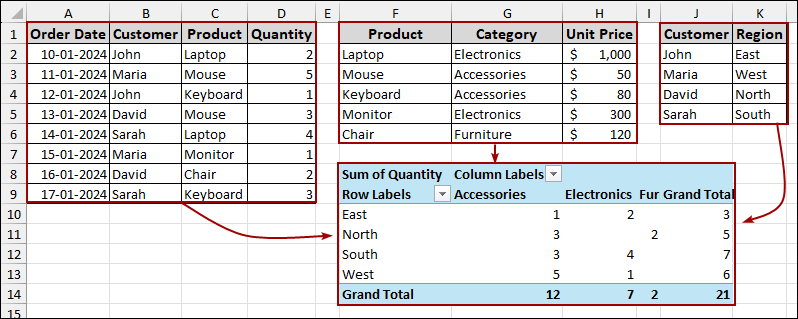
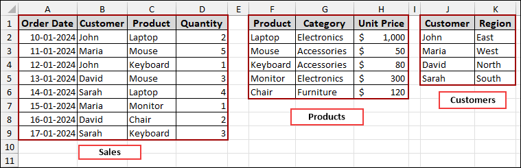
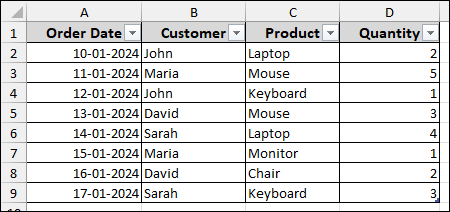
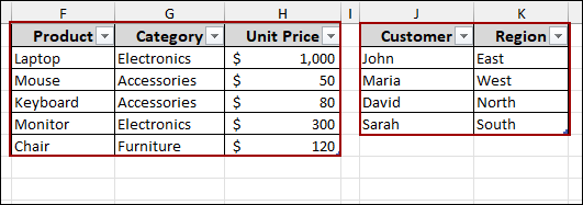
Suppose we have data for “Sales”, “Products”, and “Customers” spread across our sheet. Now, we will prepare the data first and then create data model relationships for these three types of data.
Step 1: Creating and Naming Tables
To begin, you need to organize your raw data into structured tables and name them. This step is crucial as it connects the tables with the data model.
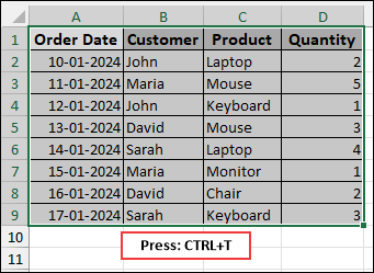
➤ Select cells from Sales data range.
➤ Press Ctrl + T to open the Create Table dialog box.
➤ Now, checkmark the “My table has headers” checkbox and click OK.
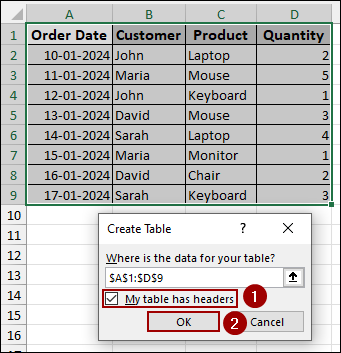
This action will convert your selected data range into an Excel table, automatically applying basic table formatting.
➤ Repeat this process for the “Products” and “Customers” data ranges as well.
Next, we will provide names to each of these newly created tables for easier identification within the data model.
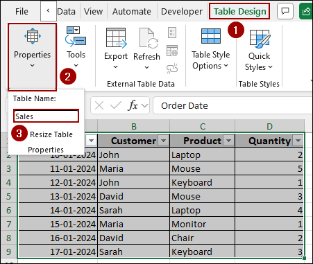
➤ Choose any cell inside your newly created Sales table and click on the Table Design tab from the menu bar.
➤ In the Properties group, choose the Table Name field.
➤ Change the default table name to Sales and press ENTER.
Repeat this process for your “Products” table, renaming it to Products, and for your “Customers” table, renaming it to Customers. These named tables will now be ready for use in the data model.
Step 2: Creating Pivot Table
Here, we will create a Pivot Table and add our data to the data model.
➤ Click on Insert > Tables > From Table/Range.
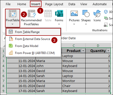
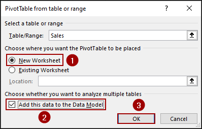
A dialog box named PivotTable from table or range will appear.
➤ Select New Worksheet to place your PivotTable on a new sheet.
➤ Checkmark the box Add this data to the Data Model and hit OK.
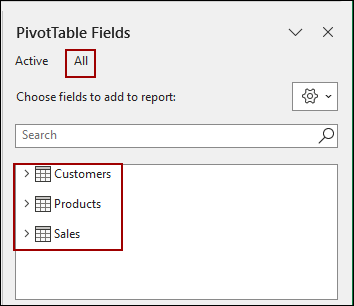
Thus, a new worksheet will open with an empty PivotTable and the PivotTable Fields pane. You will observe that under the “All” tab in the PivotTable Fields pane, all your named tables (Customers, Products, Sales) are listed.
Step 3: Adding Relationships Between Tables
In this part, we will define relationships between the tables. Thus, the three tables will be connected, allowing you to analyze data in a single Pivot Table.
➤ From the PivotTable Analyze tab, in the Calculations group, click on Relationships.
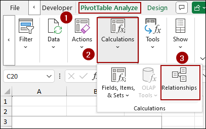
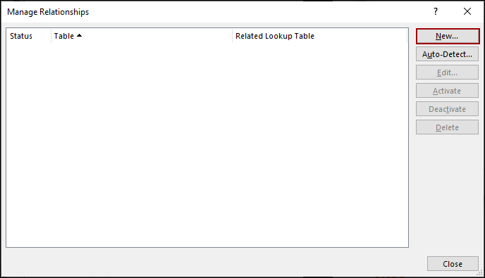
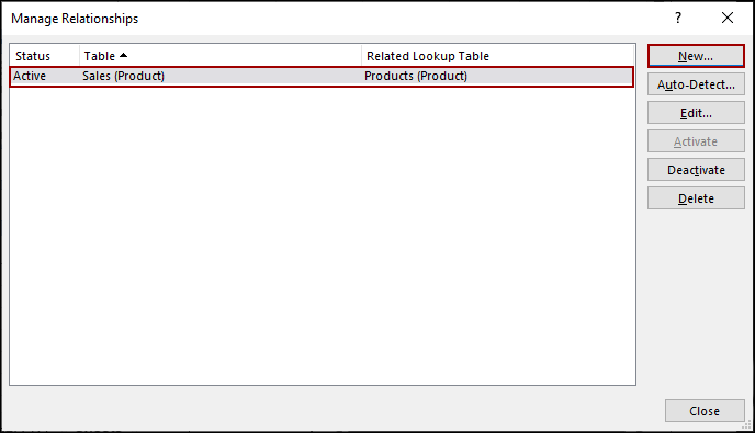
This will open the Manage Relationships dialog box.
➤ Click on the New button.
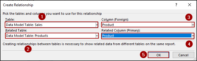
In the Create Relationship dialog box, you will define the connection between your “Sales” and “Products” tables.
➤ In the Table dropdown, choose Data Model Table: Sales.
➤ In the Column (Foreign) dropdown, choose Product.
➤ In the Related Table dropdown, choose Data Model Table: Products.
➤ In the Related Column (Primary) dropdown, choose Product.
➤ Click OK.
This way, the first relationship (Sales (Product) > Products (Product)) will be added to the Manage Relationships dialog box.
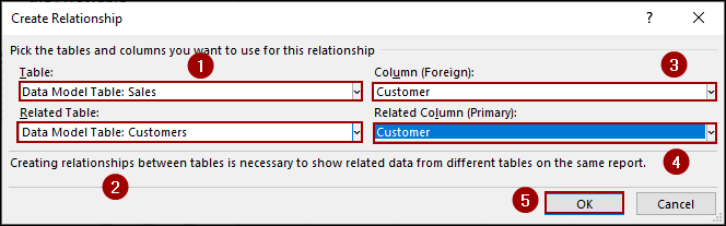
Now, we will add the second relationship between “Sales” and “Customers”.
➤ Click on the New button again.
➤ In the Table dropdown, choose Data Model Table: Sales.
➤ In the Column (Foreign) dropdown, choose Customer.
➤ In the Related Table dropdown, choose Data Model Table: Customers.
➤ In the Related Column (Primary) dropdown, choose Customer.
➤ Click OK.
Thus, both relationships will be listed in the Manage Relationships dialog box.
Step 4: Building Pivot Table
Finally, with our tables organized and their relationships established, we will move towards building the Pivot Table.
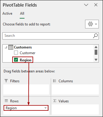
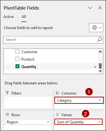
In the PivotTable Fields pane:
➤ From the Customers table, drag the Region field to the Rows area.
➤ Similarly, from the Products table, drag the Category field to the Columns area.
➤ Then, from the Sales table, drag the Quantity field to the Values area.
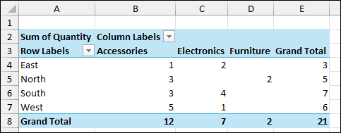
As a result, your Pivot Table will now display the Sum of Quantity for each Region (from the Customers table) broken down by Category (from the Products table). This demonstrates the successful integration of data from multiple tables through defined relationships.
Frequently Asked Questions
Why should I use relationships instead of VLOOKUP?
Relationships allow you to connect tables without using formulas like VLOOKUP. It is easier to manage and supports many-to-one or one-to-one relationships.
Can I create relationships using more than one column?
No, Excel’s built-in data model only supports relationships based on a single column in each table. For composite keys, use Power BI or Power Pivot.
What happens if the relationship column has duplicates on both sides?
Excel relationships require that one of the tables have unique values in the relationship column. If both sides have duplicates, the relationship will fail.
Concluding Words
Above, we have explored step by step process to create and use relationships in Excel’s data model to connect multiple tables and analyze them through a Pivot Table. This approach makes it simple to work with large datasets and create reports with just a few clicks. If you have any questions, feel free to leave them in the comments below.