In financial accounting, a ledger is an important tool that helps to track financial transactions. After creating a primary journal, separate ledgers are created for different accounts to know the exact balance of those accounts. Excel makes it easy to create a ledger with its spreadsheets.
In this article, we will learn how to make a ledger in Excel. We will start with a journal, and import the transactions that we need to prepare the ledger. If you follow the guide thoroughly, you will be able to create ledgers for your business as well.
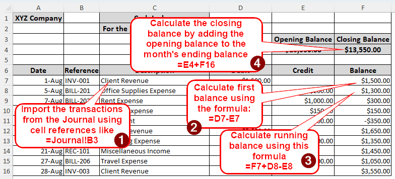
➤ First, import the transactions that are related to the ledger from the journal using the following formula for each cell:
=Journal!B3
➤ Replace Journal with the Journal sheet, and B3 with the cell reference.
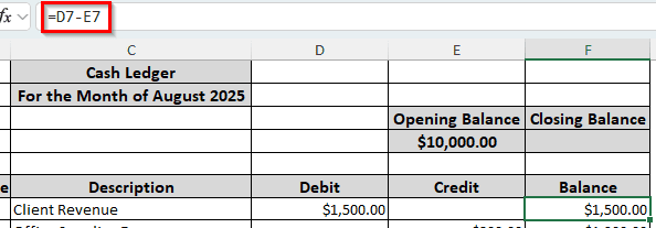
➤ Calculate the balances of the first transaction using the formula from below:
=D7-E7
➤ Replace D7 with the debits and E7 with the credits. If it’s not an asset ledger, the debits and credits will swap places.
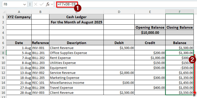
➤ Calculate the running balance for the rest of the cells using the following formula, and autofill the rows if you need:
=F7+D8-E8
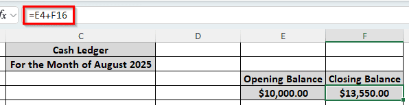
➤ Calculate the closing balance with this formula: =E4+F16
➤ Use the opening balance for E4 and the ending running balance for F16.
Creating a ledger is no easy job, but we can make it simpler for you. The step-by-step guide we prepared for you will give you a clear idea of how to make a ledger for your company or business. Read the article attentively, and check every step so that you make no mistakes.
Steps for Making a Ledger in Excel
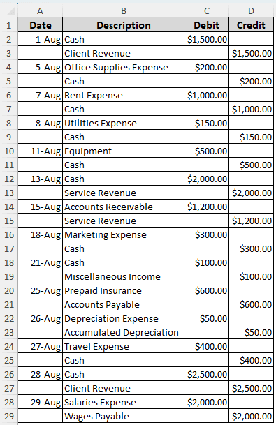
Before starting to make a ledger, we need a journal to import the transactions from. Here, we have the journal for August 2025 with a bunch of transactions. We will make a cash ledger, so we are only interested in the transactions that include cash. Let’s start with the ledger creation process:
Step 1: Prepare the Format
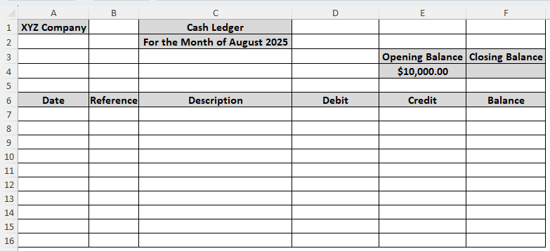
➤ We need to create a table with six columns. The column headings are Date, Reference, Description, Debit, Credit, and Balance.
➤ At the top, we will have the company name, the ledger name, the mention of the month, the opening, and the closing balance. The opening balance should be imported from the last month’s ledger, and we will calculate the closing balance.
➤ For those headings, we use the bold format by pressing Ctrl + B .
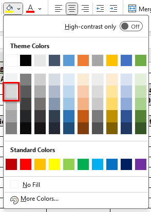
➤ To color the cells, we go to the font section of the Home tab and select the paint bucket. Then, we choose “White, Background 1, Darker 15” color properties.
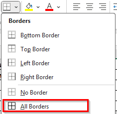
➤ For the rest of the cells, we enable All Borders from the Borders icon in the Font section of the home tab.
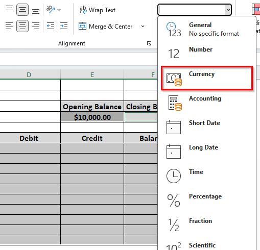
➤ Now we need to select the cells in the Debit, Credit, and Balance sections, and set them to Currency. To do so, we go to the Number section of the Home tab and open the dropdown menu to select Currency.
➤ Finally, the table should look like the following:
Step 2: Bring Over the Transactions
Now that the table is done, we need to import the transactions from the journal. Here is how to do that:
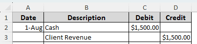
➤ The dates will be brought from the journal, and the references should be imported from the bills/vouchers, etc. We need to check each and every transaction to choose which ones to import.
➤ The first transaction is a Client Revenue. We will use the description that is named against the cash. As cash is debited, we have to put that into debit as well.
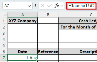
➤ In the A7 cell, write the following formula to import it from the transaction from the Journal sheet:
=Journal!A2
➤ Import the description from the B3 cell using the following formula:
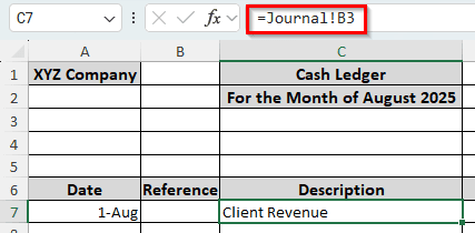
➤ Import the dollar amount by writing the following formula in the D7 cell:
=Journal!C2
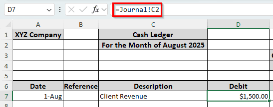
➤ Check the reference bills for the reference number and insert it in B7. Finally, the row should look like the following:
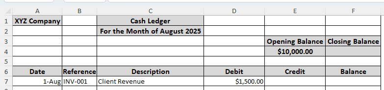
➤ Follow the process in this step for all of the transactions except the ones that do not contain cash.
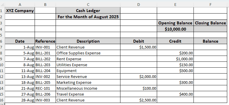
Step 3: Calculate the Balance
Now that all of the transactions have been imported, we can move on to calculating the balance. Here is how to do it:
➤ Enter the following formula in the F7 cell.
=D7-E7
➤ Use this formula for F8 cell and autofill till F16.
=F7+D8-E8
➤ Insert this formula in the F4 cell:
=E4+F16
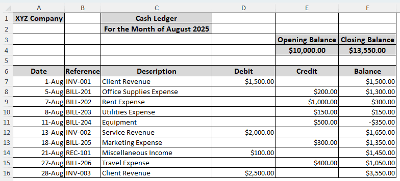
➤ At the end, the ledger should look like this:
Frequently Asked Questions
How to make a ledger PDF?
After creating your ledger in Excel, go to File > Save As. Then, select PDF format for saving the file. The ledger will be saved as PDF now.
Who prepares a general ledger?
The accountants prepare general ledgers to store transactions and organize financial data so that they can create the financial statements.
What are the five items on a ledger?
The five types of accounts that are used to create ledgers are assets, income, liabilities, expenses, and equity. These all fall into the general ledger category.
What is the difference between a balance sheet and a general ledger?
A balance sheet is created from the ledgers, and ledgers are created from journals. A ledger contains the transactions related to a single account. For example, in a cash ledger, only the transactions that involve cash will be included. In a balance sheet, all of the balances from the ledgers will be included to check whether there is an issue with the calculations or not.
What are the three main types of ledgers?
The three types of ledgers are the general ledger, sales ledger, and purchases ledger.
Wrapping Up
In this article, we have learned how to make a ledger in Excel. If you follow the tutorial properly, you too will be able to make ledgers on your own. Leave your queries regarding ledgers in the comment section, and we will try our best to provide you the solutions you need.