In the USA, the MACRS is the official method provided by the IRS for calculating depreciation of tangible properties. For novice taxpayers, it might be hard to understand the MACRS depreciation methods and prepare a depreciation schedule. In this article, we will learn all the methods you can apply to calculate MACRS depreciation in Excel. We will review the Excel functions available for calculating MACRS and discuss when to use dedicated functions versus manually calculating depreciation.
➤ Download the official IRS rates from the Pub 946 of the IRS website.
➤ Create a table for the depreciation calculation, using 1 more year than the asset’s lifetime.
➤ Multiply the asset cost by the respective IRS values from the table to calculate the MACRS depreciation.
➤ Calculate the book value by subtracting the current year’s depreciation from the previous year’s book value.

There are multiple methods of calculating MACRS depreciation. If you want to follow the law properly, you must learn all the methods and select the one that fits your business. Download the workbook of this tutorial, and get started with the methods.
What is MACRS?
MACRS, the Modified Accelerated Cost Recovery System, is the official depreciation system for properties supported by the IRS of the United States. Publication 946 of the IRS indicates the rules for calculating MACRS depreciation. There are primarily two methods of calculating according to MACRS. Those are GDS (General Depreciation System) and ADS (Alternative Depreciation System). No salvage value is considered according to the MACRS.
Calculating ADS Depreciation using the SLN Function in Excel
Among the two methods of MACRS, ADS is relatively easy to calculate. We have three pieces of information here to calculate the depreciation. There is the asset cost, the lifetime in years, and the convention to use for depreciation. Here is how to use these data to calculate the depreciation:

➤ Prepare a table for calculating the depreciation. The columns should be as follows:
Year, Depreciation, Book Value

➤ Fill the Year column with 0-11. At the half-year convention, we need to calculate depreciation for one more year than specified, because the first year starts in July. Those six months must be made up with the extra year.

➤ In the F2 cell, write the following formula:
=B1

➤ In the E3 and E13 cells, write the following formula:
=SLN($B$1,0,$B$2)/2

➤ Insert the following formula in the E4 cell, and autofill till E12:
=SLN($B$1,0,$B$2)

➤ Use the following formula in the F3 cell, and autofill the column.
=F2-E3

Using the VDB Function to Calculate GDS Depreciation in Excel
In most cases, you will have to use the generic depreciation system (GDS) to calculate the depreciation. Excel’s VDB function can be used to calculate the approximate depreciation values in the GDS method. Follow the instructions below:
➤ Create a table with the following columns:
Year, Start Period, End Period, Depreciation, Book Value
➤ Fill the Year column with 0-11 count.

➤ In the I2 cell, insert the following formula:
=B1

➤ In the F3 cell, write 0 as the first start period is from the beginning. Write the following formula in the G13 cell:
=B2

➤ In the G3 cell, insert the following formula and autofill till G12:
=E3-0.5

➤ In the F4 cell, insert the following formula and autofill the column:
=E4-1.5

➤ In the H3 cell, insert the following formula and autofill:
=VDB($B$1,0, $B$2, F3, G3)

➤ In the I3 cell, insert the following formula, and autofill:
=I2-H3

Measuring the Depreciation using Depreciation Schedules from the IRS
Full disclosure, this is the only method that you should actually use. IRS provides depreciation rates in Pub 946 that you have to use to calculate the depreciation amount. The previous method only calculates the approximate depreciation value. For proper calculation, the official depreciation rates must be used. We have modified the dataset a bit to calculate the GDS with a life-time of 7 years, as that is the most used.
The official half-year table:

Dataset:

➤ Create a table for depreciation calculation with the following columns:
Year, Depreciation, Book Value
➤ Fill the Year column with 0-8 year count. In the F2 cell for the initial book value, insert the following formula:
=B1

➤ Insert the following function in the E3 cell, and autofill the column:
=$B$1*(XLOOKUP(D3,'Half-Year Table'!$A$4:$A$11,'Half-Year Table'!$D$4:$D$11))

In that function, the first parameter is the value that it must look for, which is the year number from D3. Then, we insert the range that contains the years in the table. Finally, we enter the range from which the function should return the value.
➤ Finally, calculate the book values using the following formula in the F3 cell, and autofilling the column:
=F2-E3

Frequently Asked Questions
How do you calculate depreciation in Excel?
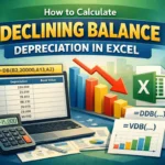
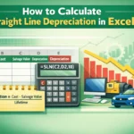
There are five functions that you can use to calculate depreciation in Excel. For declining balance methods, you have three functions: DB, DDB, and VDB. To calculate straight-line depreciation, you can use the SLN function. Finally, to calculate the depreciation using the sum of years’ digits method, you can use the SYD function.
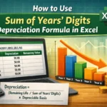
What is the SYD function in Excel?
The SYD function helps calculate the accelerated depreciation of a property using the sum of years’ digits method. The function requires four parameters. The syntax of the function is as follows:
=SYD(cost, salvage, life, period)
You can use cell references or numeric values. The first three parameters are self-explanatory. The fourth parameter refers to the year for which the depreciation is being calculated.
What is the depreciation rate for a 5-year effective life?
In general, the depreciation rate for a 5-year asset should be 100/5=20%. However, businesses might have salvage values of the asset, in which case, you might want to change the rate accordingly. You should use the rate according to the rules of in-house accounting.
Which depreciation method is best?
There is no best depreciation method; it always depends on the choice of the company and what fits best with their practices. However, the most used depreciation method is the straight-line depreciation method, where the depreciation remains the same for every year.
What are the IRS guidelines for depreciation?
Please follow the publication 946 to depreciate your property. In general, the guidelines indicate that the property must be your own, used by an income-producing activity, have a determinable useful life, and last more than a year.
Wrapping Up
In this article, we learned how to calculate MACRS depreciation in Excel. We have learned different methods we can use in Excel, and when to use what method. To follow the exact guidelines of calculating MACRS depreciation according to the US IRS, please follow Pub 946. Always keep updated on the depreciation guidelines to avoid legal issues.