If you are a retailer or distributor who works with sales units, you might need to calculate the total sales of your products. While most people prefer using the SUM function, there are actually several other methods to calculate total sales. Depending on the complexity of your data and your needs, you will have to choose different methods to calculate the sales data in your spreadsheet. In this article, we will learn all of the ways you can calculate the total sales in Excel.
➤ Use the following formula and autofill the table to calculate the total sales of each item:
=B2*C2
➤ Replace B2 with the untis sold and C2 with the revenue.
➤ To calculate the total sales revenue, adapt the following formula:
=SUM(D2:D5)
➤ Replace D2:D5 with the range of the total sales of each item.

That was a simplified version of how the total sales calculation works, but we have four detailed methods in this tutorial. It is up to you to learn the methods and choose the one that best fits your dataset.
Using the SUM Function to Calculate the Total Sales
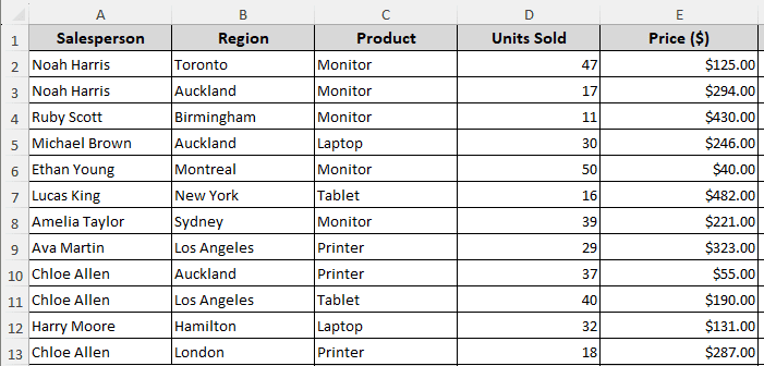
We have a dataset with some salesperson names, their regions, the products they sell, the number of units they sold, and the price of each unit. We will calculate the total sales from these values.
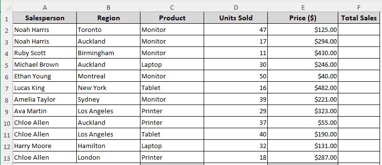
➤ First, add a new column for calculating the total sales for each row.
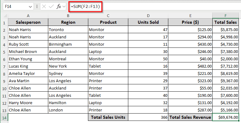
➤ Insert the following formula in F2 and autofill till F13:
=D2*E2
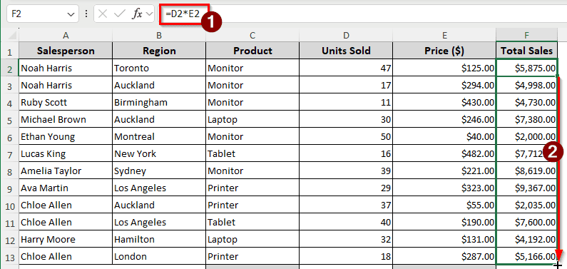
We are multiplying the units sold (D2) by the price (E2) to calculate the total sales for the row.
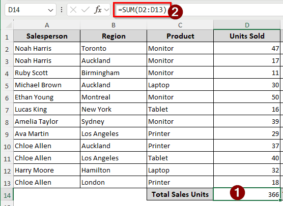
➤ To calculate the total sales unit, use the following formula in the D14 cell:
=SUM(D2:D13)
➤ Calculate the total sales revenue using the following formula in the F14 cell:
=SUM(F2:F13)
Finding the Total Sales of Each Product Using the SUMIF Function
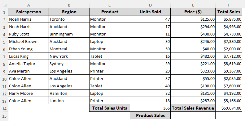
We know how to calculate the total sales of all the products. But what if we wanted to find the total sales or each product or salesperson? Follow the instructions below to learn how to do so:
➤ We start with the table we prepared in the previous method. Add another row to calculate the product sales.
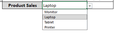
➤ Click on the E15 cell. From the Data tab on the ribbon, go to Data Tools > Data Validation.

➤ In the new window, we should be by default on the Settings tab. From Allow, select List, and write this in the Source box:
=$C$2:$C$13
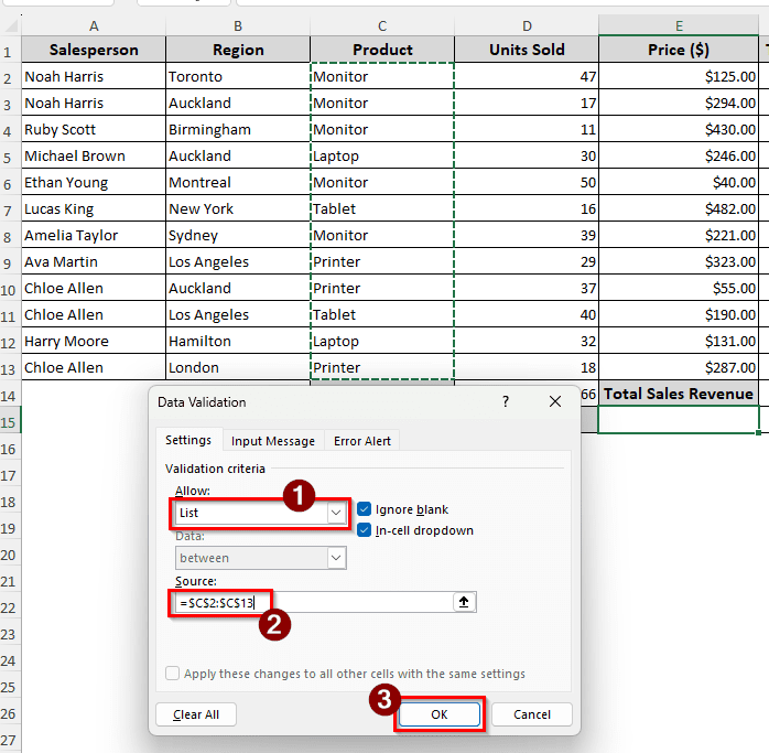
This is the range of the products that we will use to filter the sums.
➤ After pressing OK, we can select an individual product from the dropdown in the E15 cell.
➤ Now, in the F15 cell, enter the following formula:
=SUMIF(C2:C13,E15,F2:F13)
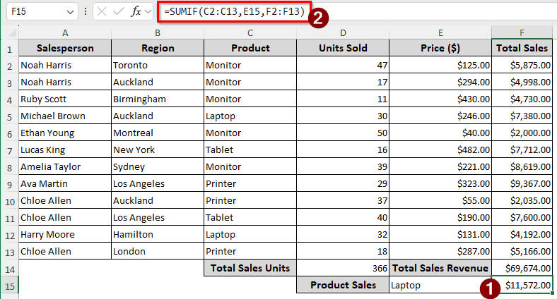
➤ Now we can select different products from the dropdown in the E15 cell, and the total sales of that product will be shown in the F15 cell automatically.
Applying the SUMPRODUCT Function to Calculate the Total Sales
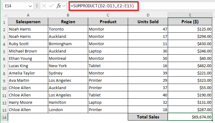
Instead of adding a separate column to calculate the sales of each row, we can use the SUMPRODUCT function to do it in one go. Follow the steps below to do so:
➤ In the E14 cell, enter the following formula:
=SUMPRODUCT(D2:D13,E2:E13)
Making Use of a PivotTable to Calculate the Total Sales
The pivot table can be a powerful method to calculate the total sales. This method is a little unorthodox, but if you learn it, it has the potential to be your favorite method from this tutorial.
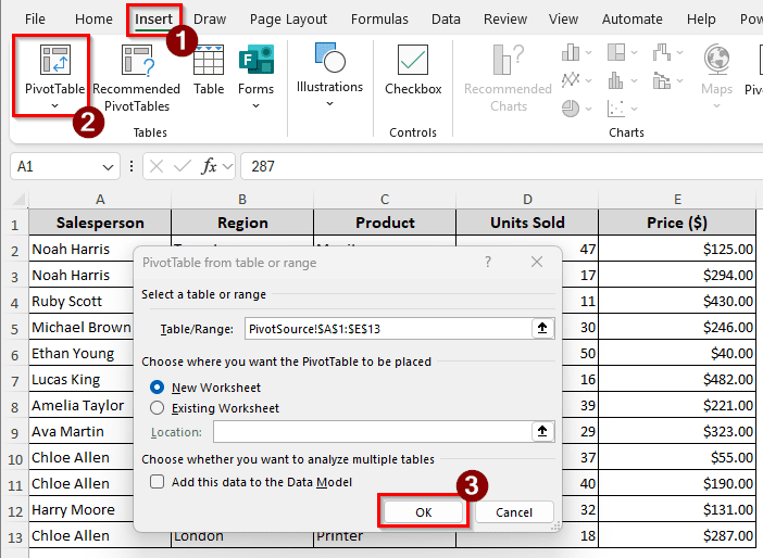
➤ Select the whole table, and go to the Insert tab in the ribbon. Click on PivotTable from the Tables group, and a small window will appear. Click OK to create the new pivot table.
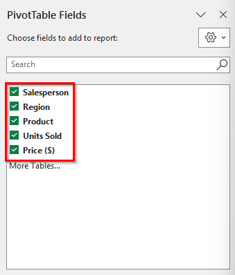
➤ In the new sheet, select all the checkboxes from the PivotTable Fields section.
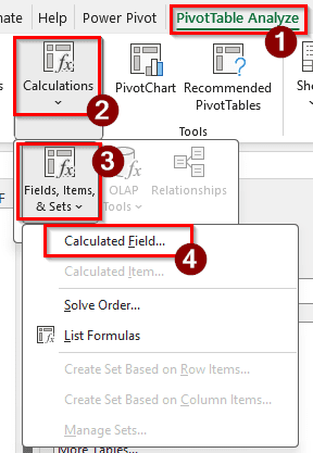
➤ Select any cell of the pivot table to enable the pivot table-related tabs on the ribbon. Then, from the PivotTable Analyze tab, go to Calculations > Fields Items, & Sets > Calculated Field.
➤ In the Insert Calculated Field window, insert Sales in the Name box, and the following formula in the Formula box:
= 'Units Sold' * 'Price ($)'
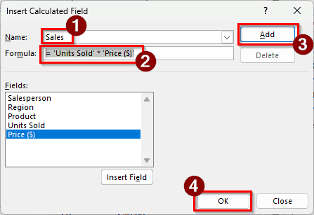
We can use the column headers to multiply the cells in a calculated field.
➤ Press Add and OK afterwards.
➤ From the Design tab, go to the Layouts group, and do two things.
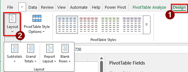
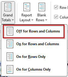
➤ First, go to Grand Totals, and select Off for Rows and Columns.
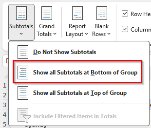
➤ From the Subtotals, select Show all Subtotals at Bottom of Group.
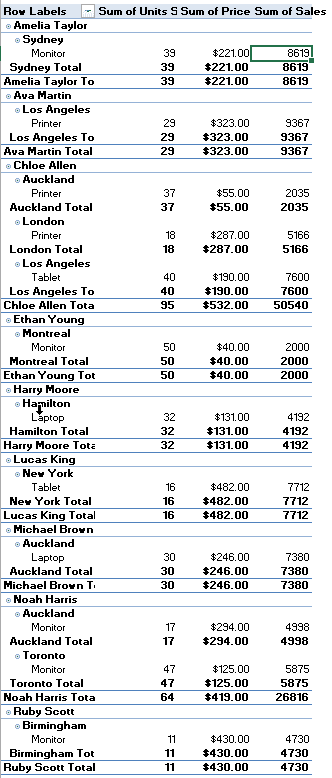
➤ Now the total sales of each salesperson are visible in the pivot table.
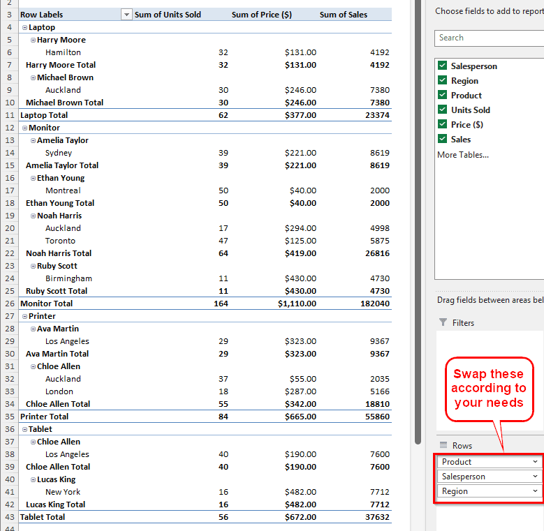
➤ We can change the order in the Rows section to see product or region-wise sales as well.
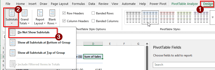
➤ To calculate the total sales of everything, first turn the subtotals off from Design > Subtotals > Do Not Show Subtotals.
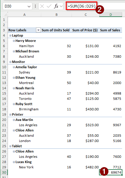
➤ Insert the following formula in the D30 cell to calculate the total sales:
=SUM(D6:D29)
Frequently Asked Questions
How do you calculate total net sales?
Net sales, unlike total sales, include some deductions to get the final revenue from sales. Total sales can be compared to gross sales, which include everything that is relevant and irrelevant to the revenue. To calculate the net sales, you can use the following formula:
=A2-(B2+C2+D2)
Here, A2 is the total sales, B2 is the sales returns, C2 is the allowances, and D2 is the discounts.
How do you calculate a sale?
A “sale” is a discount provided on a product for promotion or some other purpose. If you subtract the discount amount from the price, you get the sale price. Here is the Excel formula to do so:
=A2-(A2*10%)
In this formula, A2 is the original price, and 10% is the amount of discount.
What is ∑ in Excel?
That is the AutoSum icon in Excel. When you click on that button in Excel, it automatically chooses a suitable range for you to sum and inserts the SUM function with appropriate parameters for you.
What is the percentage of total sales?
The total sales percentage formula is as follows:
=A2/B2
Here, A2 is the number of items you have sold, and B2 is the number of items you had to sell. Set the cell format to percentage to see the results as intended.
How to calculate 10% of sales?
Just multiply the sales value by 10% or 0.1 to calculate 10% of sales. In Excel, the formula will be as follows:
=A2*0.1
In this case, the A2 cell has the sales value.
Wrapping Up
In this article, we have learned four methods to calculate total sales in Excel. We have all the formulas and the dataset in the practice Excel file that can be downloaded free of cost. If you can take a moment, please leave your feedback. We love hearing from you. For more Excel tutorials, bookmark the site and give us a visit now and then.