
The Fisher test evaluates any significant association between two categorical variables. We can perform the Fisher test in Excel using the HYPGEOM.DIST function to get the one-tailed and two-tailed P values.
➤ Fisher test determines any association between two categorical variables. In this article, we’ll learn about Fisher’s exact test and how we can calculate the one-tailed and two-tailed P values using the HYPGEOM.DIST function.
➤ To calculate one-tailed P value: =HYPGEOM.DIST(sample_s, number_sample, population_s, number_pop, cumulative)
➤ To calculate two-tailed P value: =HYPGEOM.DIST(sample_s1, number_sample, population_s, number_pop, cumulative)+1-HYPGEOM.DIST(sample_s2, number_sample, population_s, number_pop, cumulative)
➤ Reject the null hypothesis if the Fisher test P value is less than the significance level.
➤ Fisher test is applicable when cell values and cell counts are small.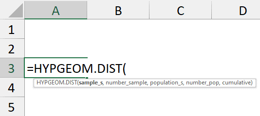
What is Fisher Test in Statistics?
The Fisher test or Fisher’s exact test determines any non-random associations between two categorical variables. Unlike the Chi-Square test, Fisher’s exact test is applicable for small sample sizes.
A typical Fisher’s exact test has the following hypothesis:
Null hypothesis: The two categorical variables are independent.
Alternate hypothesis: They are not independent.
HYPGEOM.DIST Function
The HYPGEOM.DIST function returns hypergeometric distribution. But we can use it to calculate the P value of Fisher’s exact test. For earlier versions of Excel, you can use the HYPGEOMDIST function.
Syntax
The syntax for the HYPGEOM.DIST function is given below. It takes 5 mandatory arguments.
=HYPGEOM.DIST(sample_s, number_sample, population_s, number_pop, cumulative)Here is the syntax for the earlier version of this function.
=HYPGEOMDIST(sample_s, number_sample, population_s, number_pop)
➤ sample_s: number of successes present in the sample
➤ number_sample: size of the sample
➤ population_s: number of successes present in the population
➤ number_pop: size of the population
➤ cumulative: TRUE returns the cumulative distribution function while FALSE returns the probability distribution function
Fisher Test vs Chi-Square Test
The Chi-Square test should be used for larger cell values and cell counts.
The Fisher test is suitable when:
➤ Cell count is less than 20.
➤ Expected cell value is less than 5.
➤ The row and column marginal values differ greatly.
Example of Fisher’s Exact Test in Excel
Consider the two-by-two contingency table comparing the success and failure of treatment A and treatment B. The two hypotheses are stated below:
Null hypothesis: The success and failure of treatments A and B are independent.
Alternate hypothesis: The success and failure of treatments A and B are not independent.
Steps:
➤ Select the output cell (C6) and enter the formula to get the one-tailed P value.
=HYPGEOM.DIST(B2,$B$4,$D$2,$D$4,TRUE)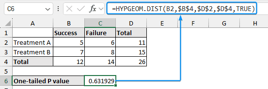
➤ To calculate the two-tailed P value use the formula below.
=HYPGEOM.DIST(B2,$B$4,$D$2,$D$4,TRUE)+1-HYPGEOM.DIST(B3,$B$4,$D$2,$D$4,TRUE)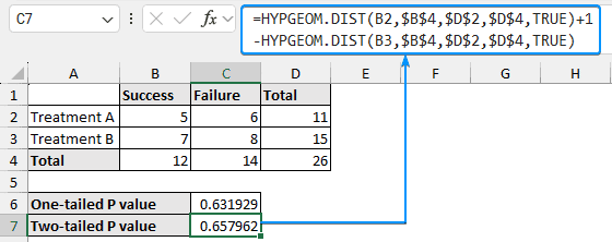
Wrapping Up
In this quick tutorial, we’ve learned about the Fisher test and we can calculate the one-tailed and two-tailed P values using the HYPGEOM.DIST function in Excel. Feel free to download the practice file and share your thoughts in the comments below.