Sometimes in Excel, you may need to add up numbers based on more than one condition in the same column. For example, if you have a list of product sales and you want to calculate the total sales for both Apple and Banana, it’s not as simple as using a regular SUMIFS formula. That’s because SUMIFS works best when the conditions are in different columns, not in the same one.
In this article, we’ll learn how to apply a formula that handles multiple criteria from the same column. This is a helpful technique when you want to group and total values for multiple products, categories, or names.
Here’s how to apply the SUMIFS function with multiple criteria in the same column:
➤ Open your dataset in Excel.
➤ Click on cell F4 to calculate the total sales for Apple and Banana.
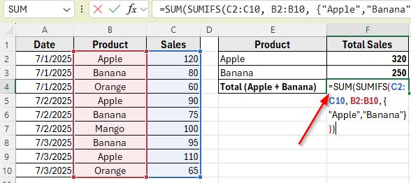
➤ Type this formula:
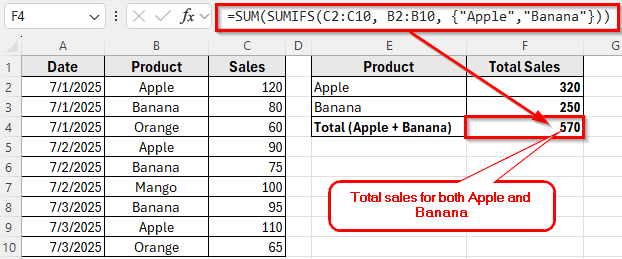
=SUM(SUMIFS(C2:C10, B2:B10, {“Apple”,”Banana”}))
➤ Press Enter.
➤ This formula adds all sales where the Product column contains either Apple or Banana.
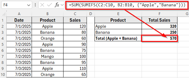
➤ Press Enter, it returns a total of: 120 + 90 + 110 (Apple) + 80 + 75 + 95 (Banana) = 570.
Using SUMIFS with Multiple Criteria in Same Column
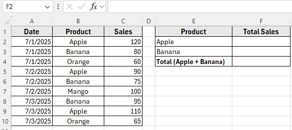
In the following dataset, we have a product sales list that includes the sale date, product name, and the sales amount for each item. There are three main columns: Date, Product, and Sales. Column A shows the date of sale, Column B lists the product names like Apple, Banana, and Orange, and Column C shows the corresponding sales figures.
We’ll use this dataset to calculate the total sales for each product keyword listed in Column E. The goal is to sum the values in Column C only if the product name in Column B matches the keyword from Column E. Column F is currently empty and will be used to display the total sales for Apple, Banana, and the combined total of both.
The standard SUMIFS function allows you to apply multiple conditions, but only when those conditions apply to different columns. When your conditions are in the same column, SUMIFS doesn’t support OR logic directly. That’s why we wrap it inside a SUM function and use an array constant to list multiple criteria.
In this method, we’ll first calculate the total sales for Apple, then for Banana, and finally use one formula to return the total for both products combined.
Here’s how to apply this formula step by step:
Step 1: Calculate Total Sales for Apple and Banana Separately
We’ll use the SUMIFS function to calculate each product’s sales based on the values in Column B and Column C.
➤ Open your dataset in Excel. First, let’s write the formula to calculate the total sales for Apple.
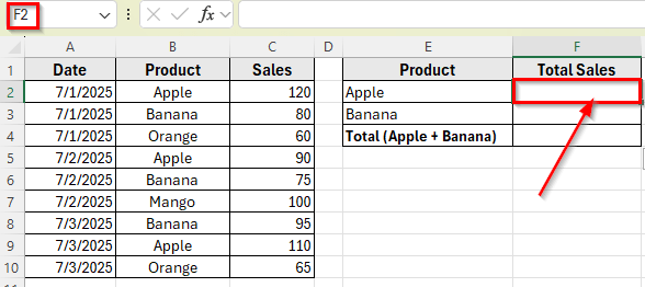
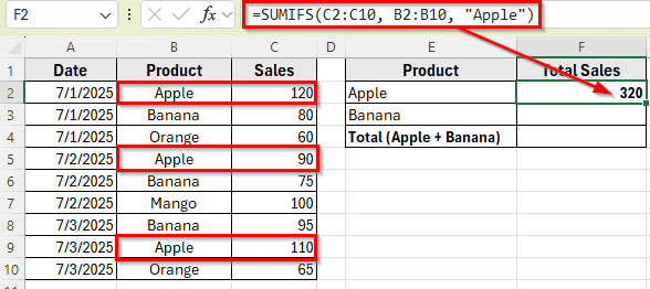
➤ Click on cell F2.
➤ Now, enter this formula
=SUMIFS(C2:C10, B2:B10, “Apple”)
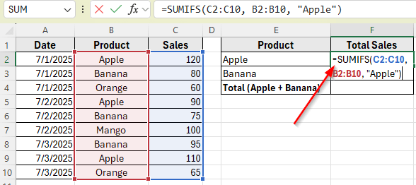
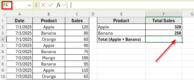
➤ Press Enter. This will return the total sales of Apple, and that is 320. For example: 120 + 90 + 110 = 320
➤ Next, click on cell F3 to write the formula to calculate the total sales for Banana.
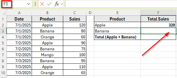
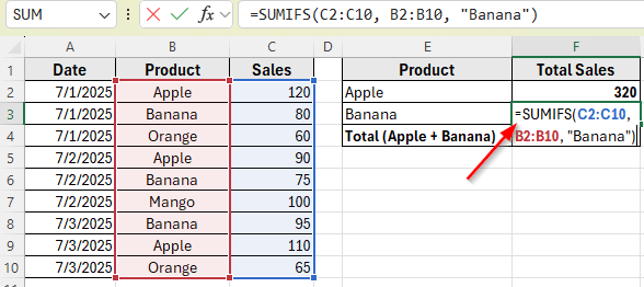
➤ Enter this formula
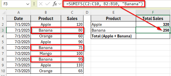
=SUMIFS(C2:C10, B2:B10, “Banana”)
➤ Press Enter. This will return the total sales of Banana, which is 250. For example: 80 + 75 + 95 = 250
Step 2: Combine Both Totals in One Formula
Now that we know how to calculate each product separately, we can combine both conditions into one formula using an array inside SUMIFS.
➤ Select cell F4, where we want to add the total sales where the Product is either Apple or Banana.
➤ Enter the following formula
=SUM(SUMIFS(C2:C10, B2:B10, {“Apple”,”Banana”}))
➤ Press Enter. This formula adds both Apple and Banana sales together and returns. For example: 320 + 250 = 570
Combine SUMIFS with SUMPRODUCT Function
Another useful way to sum values based on multiple criteria in the same column is to combine the SUMIFS logic with the SUMPRODUCT function. This method gives you more flexibility, especially when you want to reference a list of product names instead of typing them directly into the formula.
Since, we already have the totals of Apple and Banana separately using the SUMIFS function, we can now use a single formula to combine both results at once by referring to the product names listed in Column E.
Here’s how to apply this method:
➤ Open your dataset in Excel.
➤ Since the totals for Apple and Banana are already calculated in cells F2 and F3, we’ll now combine them into a single formula.
➤ Click on cell F4, where you want to show the combined total.
➤ Type the following formula
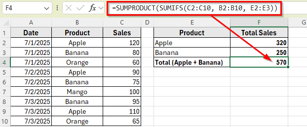
=SUMPRODUCT(SUMIFS(C2:C10, B2:B10, E2:E3))
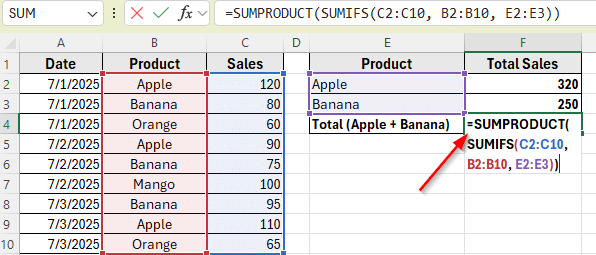
➤ Press Enter. This will return the final result: 570, which is the total sales for both Apple and Banana. For example: 120 + 90 + 110 (Apple) + 80 + 75 + 95 (Banana) = 570.
Frequently Asked Questions
How to use SUMIFS with multiple criteria in the same column?
To apply SUMIFS with multiple conditions in the same column, use an array formula like this:
=SUM(SUMIFS(sum_range, criteria_range, {“Item1″,”Item2”}))
Such as =SUM(SUMIFS(C2:C10, B2:B10, {“Apple”,”Banana”}))
This formula checks the criteria range for each item listed in the array and adds the corresponding values. It’s a simple way to apply OR logic across a single column using SUMIFS.
Why is SUMIFS with multiple criteria not working?
If your SUMIFS formula isn’t working, it’s usually because the ranges in the formula don’t match in size. The range you want to sum and each criteria range must have the same number of rows.
Another common mistake is trying to check for more than one value in the same column using normal SUMIFS logic.
For example, if you use =SUMIFS(C2:C10, B2:B10, “Apple”, B2:B10, “Banana”), it won’t work because a single row can’t be both Apple and Banana at the same time. To fix this, use an array like =SUM(SUMIFS(C2:C10, B2:B10, {“Apple”,”Banana”})) to apply both conditions properly.
Wrapping Up
When you need to sum values based on multiple criteria in the same column, Excel offers simple and effective solutions. Using SUMIFS function with an array constant or combining SUMIFS with SUMPRODUCT function lets you add numbers for several conditions at once without extra helper columns.
These formulas update automatically when you change the criteria list, making your calculations flexible and easy to manage. Try these methods to see which one works best for your data and use them to simplify your Excel tasks.