Blank cells within an Excel Pivot Table often occur when there is no data entry for a specific row and column labels. These blanks can make data analysis and reporting confusing. Fortunately, Excel offers several methods to manage or remove these blank values. In this article, we will guide you through four effective methods for removing blanks from Pivot Table: using the Filter tool, applying the Find and Replace feature, adjusting Pivot Table options for numeric values, and utilizing a Slicer.
To remove blank from Pivot Table, here is one simple solution by using the Filter tool.
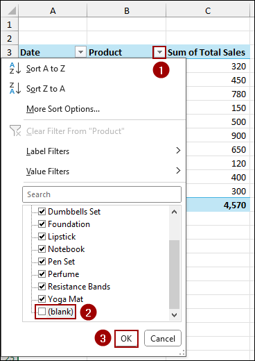
➤ Click the Filter icon from the column header (e.g., “Product”) where the blank entries appear.
➤ Remove the checkmark from the Blank box.
➤ Press OK, and you will see the blank cells are removed from the Pivot Table.

Removing Blanks from Pivot Table Using Filter Tool
The easiest way to remove visible blank entries from a Pivot Table is by using the built-in Filter tool. Here, we will use the Filter icon to remove blanks from the product label.
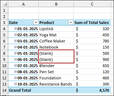
Consider a sample Pivot Table that contains blank entries in the “Product” column.
➤ Click the Filter dropdown arrow next to the column header (e.g., “Product”) where the blank entries appear.
➤ In the list of items, scroll down to the bottom and uncheck the box labeled blank.
➤ Click OK to apply the filter.
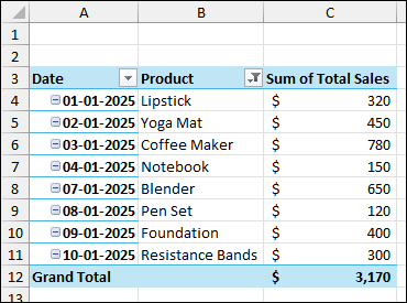
As a result, the Pivot Table will immediately update, removing blank values from the Pivot Table.
Using Find and Replace Window to Remove Blanks
If you prefer to replace the blank cells with a specific text or value (like “N/A” or “No Data”) instead of removing the entire row, you can use the Find and Replace feature. This method is useful for quickly standardizing the appearance of missing data across the entire Pivot Table.
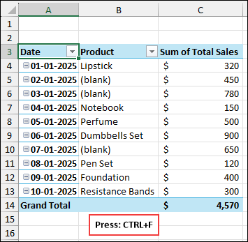
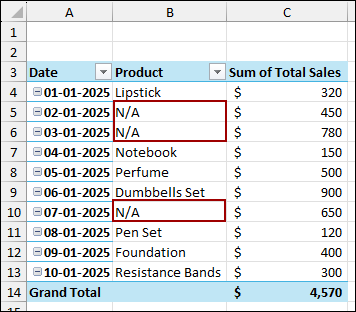
Imagine the Pivot Table with the blank cells in the Product label.
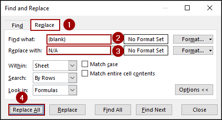
➤ Press Ctrl + F on your keyboard to open the Find and Replace dialog box.
➤ Go to the Replace tab.
➤ In the Find what field, type (blank).
This is the text Excel uses to display a blank cell within a Pivot Table.
➤ In the Replace with field, enter the text you want to use, such as N/A.
➤ Click Replace All.
Excel will replace all instances of “(blank)” with your chosen text. Your Pivot Table now clearly shows “N/A” where the data was missing.
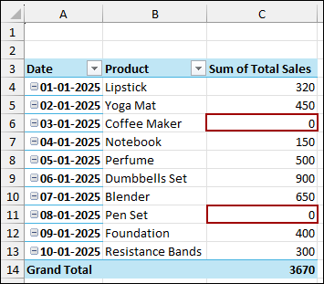
Utilizing Pivot Table Options to Remove Blanks with Numeric Values
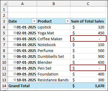
When blank cells appear in the Values area of your Pivot Table (e.g., the “Sum of Total Sales” column), it’s typically because the source data had a blank or zero. You can use the Pivot Table Options for numeric fields to remove the blanks.
Imagine the same Pivot Table having blanks in the Sum of Total Sales label.
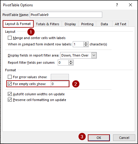
➤ Right-click anywhere inside the Pivot Table.
➤ From the context menu, select PivotTable Options.
![]()
➤ In the PivotTable Options dialog box, ensure the Layout & Format tab is selected.
➤ Under the Format section, checkmark the box For empty cells show.
➤ In the input field, enter the value 0 to display.
➤ Click OK.
The Pivot Table will now display a 0 instead of a blank cell for any missing numeric values.
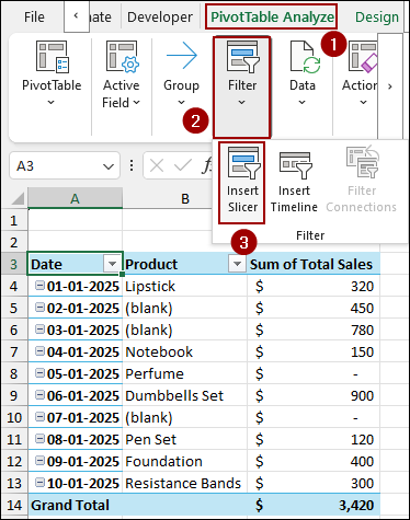
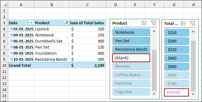
Applying Slicer to Remove Blank from Pivot Table
Slicers are used to filter Pivot Table data in Excel. They also provide a simple method to filter out blanks from your Pivot Table’s row or column labels.
➤ Select any cell within your Pivot Table.
➤ Go to the PivotTable Analyze tab on the ribbon.
➤ In the Filter group, click Insert Slicer.
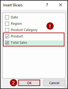
➤ The Insert Slicers dialog box will appear.
➤ Checkmark the box for the field you want to filter, such as Product or Total Sales.
➤ Click OK.
The Slicer will display buttons for every unique item in that field, including a dedicated button labeled (blank).
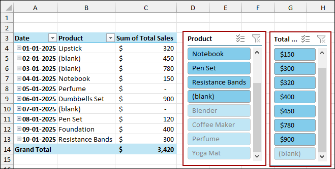
To remove the blank entries:
➤ Click on all other buttons except the (blank) button to manually exclude it from the filter selection.
As a result, you will get a clean Pivot Table removing blanks.
Frequently Asked Questions
Does using the Filter tool to hide blanks change the source data?
No. Filtering a Pivot Table only changes the view of the data within the Pivot Table itself. The source data is left completely untouched.
Why does the Find and Replace method not work when my Pivot Table uses a Data Model?
The Find and Replace feature is designed for cell content, but Pivot Table content from a Data Model is dynamic and often not directly replaceable. You can use the Pivot Table Options for numeric blanks, or filter the source table before creating the Data Model.
Why does my Pivot Table show an empty cell in the Values area even though I typed “0” in the ‘For empty cells show’ box?
The cell might contain a non-numeric error value from the source data. Ensure you check the box and enter “0” in the ‘For error values show‘ box as well, or correct the source data errors.
Concluding Words
Above, we have explored several ways to remove blank from Pivot Table. While filtering is the fastest solution for removing blank rows, using the PivotTable Options is essential for replacing numeric blanks with 0. Furthermore, the Find and Replace feature offers flexibility for replacing text-based blanks, and Slicers provide an interactive filtering experience. If you have any questions, please don’t hesitate to share them in the comments section below.