Pivot Tables focus on summarizing data in Excel. While they provide standard aggregation methods like Sum and Count, sometimes you need a more advanced calculation, such as a conditional count or a count based on a field that doesn’t exist. This is where the Calculated Field feature becomes essential. In this article, we will guide you through using a Calculated Field to perform a specialized count in your Excel Pivot Table.
Using a Calculated Field to count in an Excel Pivot Table, here is a simple step-by-step solution.
➤ Create a helper column in the source table and enter 1 for every record.
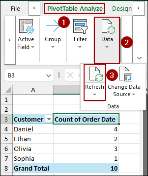
➤ Refresh the Pivot Table and go to PivotTable Analyze > Fields, Items, & Sets > Calculated Field.
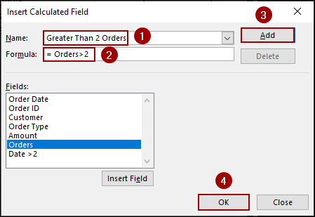
➤ Name the field as Greater Than 2 Orders, write down the formula below, and click Add.
➤ Click OK to display the proper count using the Calculated Field in Excel Pivot Table.
Steps to Get a Count Using Calculated Field in Excel Pivot Table
Here, we will create a conditional count, for example, counting which customers have placed more than two orders. We will first demonstrate why using a field already summarized as a count in a Calculated Field does not work as expected. After that, we will provide the step-by-step solution.
Step 1: Creating a Pivot Table
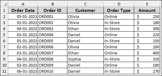
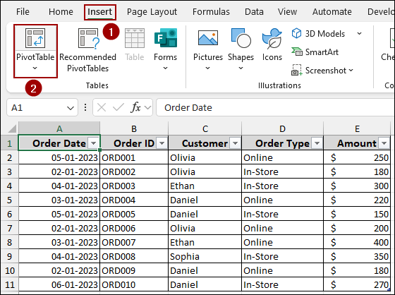
Suppose we have a dataset containing Order Date, Order ID, Customer, Order Type, and Amount. Before creating a Calculated Field, we first need a basic Pivot Table.
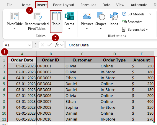
➤ Select the data, go to the Insert tab, and click Table.
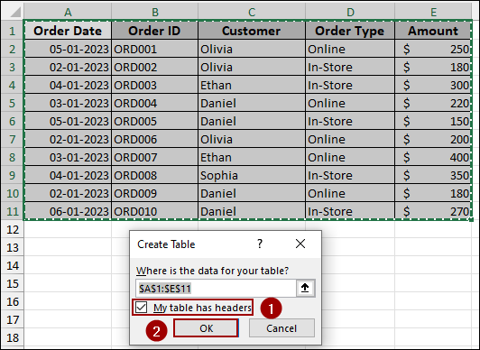
➤ In the dialog box, confirm the data range and checkmark the box for My table has headers.
➤ Click OK.
➤ Select any cell within the newly created Table.
➤ Go to the Insert tab.
➤ Click PivotTable in the Tables group.
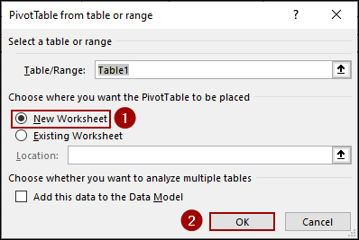
➤ In the PivotTable from table or range dialog box, select the New Worksheet option to place the Pivot Table on a clean sheet.
➤ Click OK.
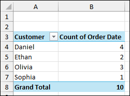
➤ In the PivotTable Fields pane, drag the Customer field into the Rows area and the Order Date field into the Values area.
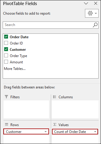
Excel will automatically default this to Count of Order Date, giving the total number of orders for each customer.
Step 2: Setting Count in the Calculated Field
Now, we will create a field that assigns a numerical value (1 or 0) based on the order count being greater than 2.
➤ Select any cell within your Pivot Table.
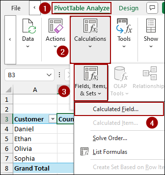
➤ Go to the PivotTable Analyze tab on the ribbon.
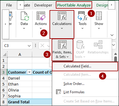
➤ In the Calculations group, click Fields, Items, & Sets, and then select Calculated Field.
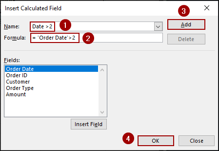
The Insert Calculated Field dialog box will open.
➤ In the Name box, type a descriptive name for the condition, such as Date > 2.
➤ In the Formula box, enter the formula.
= 'Order Date' > 2
➤ Click Add, and then click OK.
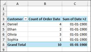
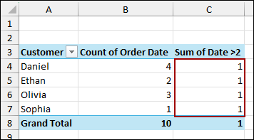
The new field, named Sum of Date > 2, will be added to the Pivot Table. As Excel’s Calculated Fields work on the sum of the data, the formula is summing the serial numbers of the dates, not the count of the orders. Thus, we will get an incorrect date format.
Step 3: Detecting Counting Error in the New Field
To view the Boolean result.
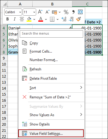
➤ Right-click on any cell in the Sum of Date > 2 column.
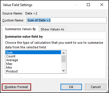
➤ Select Value Field Settings from the context menu.
➤ In the Value Field Settings dialog box, click the Number Format button at the bottom.
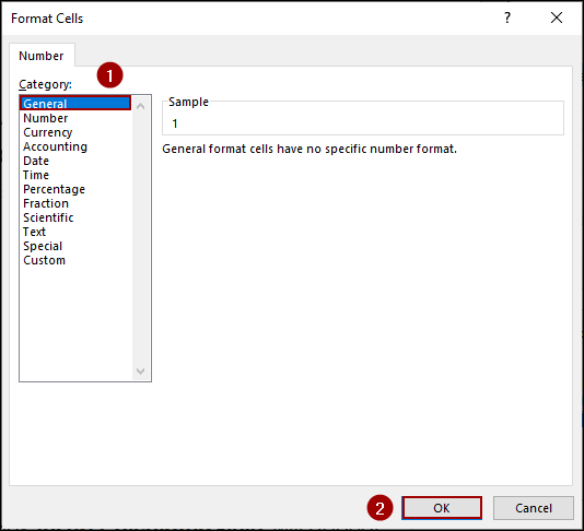
➤ In the Format Cells dialog box, select General from the Category list.
➤ Click OK on both dialog boxes.
The column now displays a 1 for every customer, which is incorrect. The Calculated Fields ignore the aggregation (count, average) and calculate based on the source data (Sum).
Step 4: Inserting Helper Column in Source Table
To overcome this limitation and get a correct conditional count, we must create a helper column in the source table.
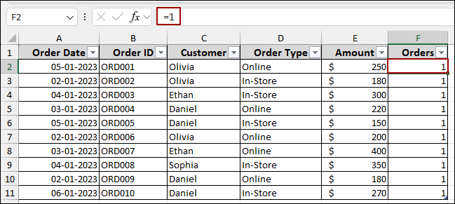
➤ In the first empty column next to the data (e.g., column F), name the header Orders.
➤ In cell F2, enter the simple formula.
=1
This formula will automatically populate the entire column with a 1 for every record. This field now acts as a reliable countable unit.
The new Orders field needs to be updated in the Pivot Table.
➤ Go back to your Pivot Table.
➤ Go to the PivotTable Analyze tab.
➤ In the Data group, click Data, and then select Refresh.
Step 5: Using Calculated Field for the Helper Column
Now, we will use the Sum of Orders for the conditional count. For this, we need to insert a new field using the Calculated Field.
➤ Select the Pivot Table, go to PivotTable Analyze, and click Fields, Items, & Sets.
➤ Choose Calculated Field.
In the Insert Calculated Field dialog box:
➤ Set the Name to Greater Than 2 Orders and enter the formula below.
= Orders > 2
Since ‘Orders‘ is a sum of ‘1‘s, this formula correctly checks if the total count is greater than 2.
➤ Click Add, and then click OK.
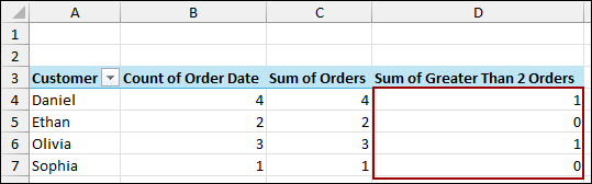
The resulting column, Greater Than 2 Orders, now correctly displays 1 for customers who meet the condition (more than two orders) and 0 for those who do not, providing the count properly in Excel Pivot Table.

Frequently Asked Questions
Do I have to keep the helper column visible in the Pivot Table after I create the Calculated Field?
No. Once the calculated field is working, you can uncheck the helper column, and the Calculated Field will continue to work correctly because it references the source data, not the visible Pivot Table fields.
Can I use the COUNT function inside a Pivot Table Calculated Field?
No, standard Excel Calculated Fields do not support the COUNT, AVERAGE, or other summary functions. They only support basic arithmetic operations (+, -, *, /) and the SUM function.
Why is the ‘Calculated Field’ option grayed out in the PivotTable Analyze tab?
This typically happens when your Pivot Table is based on the Data Model, which often occurs if you checkmark the box “Add this data to the Data Model” when creating the Pivot Table or if it uses multiple related tables. In this scenario, you can use a DAX Measure instead of a Calculated Field.
Concluding Words
Above, we have explored getting a count using Calculated Field in Excel Pivot Table. The Calculated Fields in Excel Pivot Tables only work with the SUM of source data, not the count. By creating a helper column of ‘1’s in the source data, the Calculated Field gets a numerical base to accurately calculate a count. If you have any questions, please don’t hesitate to share them in the comments section below.