When we try to analyze large datasets in Excel, pivot tables help us to summarize and analyze information quickly. However, there are situations where the built-in fields and totals are not enough. Such as when we want to combine two existing categories, compare items within the same field, or create a new group without changing the original dataset. In such cases, we need to use a Calculated Item in our pivot table.
Suppose you are analyzing sales by region with four categories including East, West, North, and South. Now, if you want to see the combined sales of East and West as a single region, you can create a Calculated Item named EastWest. This way, the pivot table will display the result as if it were a real category, even though it does not exist in our source data.
In this article, we will explain how to use a calculated item in a pivot table using the PivotTable Analyze tab.
➤ First, select your dataset and click on the Insert tab from the upper menu bar.
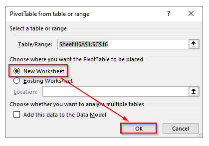
➤ Now, select PivotTable from the table option, and you will see a pop-up come out. In it, choose the New Worksheet for your pivot table to be placed. At last, select Ok.
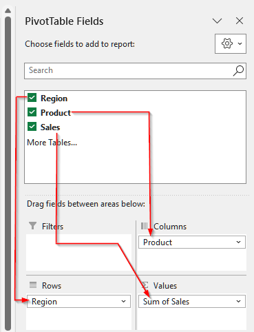
➤ Then, drag Region into Rows, Sales into Values, and the Product into the Columns field inside the PivotTable Fields pane.
➤ Now, click on one of the Region names inside your pivot table and go to the upper ribbon. From there, click on the PivotTable Analyze tab.
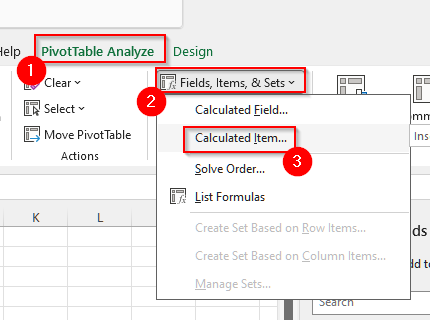
➤ Then, from the Calculations group, click on Fields, Items & Sets. You will see a list of options appear. From that list, choose Calculated Item.
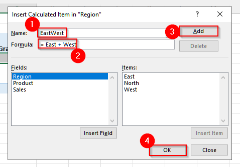
➤ Another new dialogue box called Insert Calculated Item will pop out. In it, write EastWest in the Name box.
➤ Then, in the Formula box, insert the following formula:
= East + West
➤ Finally, click Add and then select Ok.
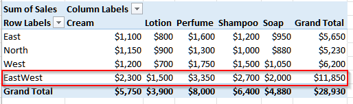
➤ Now, you will see a new row, called EastWest, appear in the pivot table. It is our calculated item.
Steps for Adding & Using Calculated Item in Pivot Table
The PivotTable Analyze tab gives us a simple way to insert a Calculated Item directly into our pivot table.
We will use the dataset below to explain how the PivotTable Analyze tab lets us use a calculated item in a pivot table.
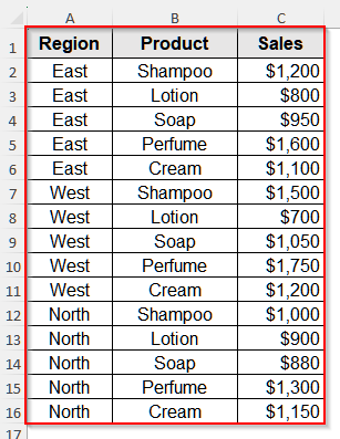
This is a regional sales dataset of a store where we have some commodities and the revenue generated by them in each region.
Step 1: Create a PivotTable
To use a calculated item in a pivot table, our first step is to make a pivot table.
Steps:
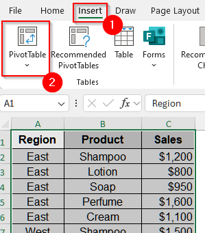
➤ First, select your dataset.
➤ Then, go to the Insert tab from the upper menu bar.
➤ Now, click on PivotTable from the table option.
➤ You will see a pop-up come out. Choose the New Worksheet for your pivot table to be placed.
➤ Finally, select Ok.
Step 2: Complete The Pivot Table
Now, we will add the relevant rows and columns to the pivot table.
Steps:
➤ First, drag Region into Rows and then, Sales into Values inside the PivotTable Fields pane.
➤ Then, drag the Product in the Columns field. Finally, the pivot table is ready.
Step 3: Insert A Calculated Item in the Pivot Table
Now, we will insert the calculated item to see the total sales revenue in the East and West regions combinedly.
Steps:
➤ First, click on one of the Region names inside your pivot table.
➤ Then, go to the upper ribbon and click on the PivotTable Analyze tab.
➤ Now, from the Calculations group, click on Fields, Items & Sets.
➤ A list of options will appear. From that dropdown, choose Calculated Item.
➤ Now, you will see a new dialogue box called Insert Calculated Item.
➤ Then, in the Name box, write EastWest.
➤ In the Formula box, insert the following formula:
= East + West
➤ Finally, click Add and then select Ok.
➤ Now, you will see a new row, called EastWest, appear in the pivot table.

Frequently Asked Questions
Why Is the Calculated Item Greyed Out or Unavailable in My Pivot Table?
The Calculated Item option for your pivot table is greyed out because the table doesn’t meet certain conditions. Usually, if all the fields are in the Values area, or if the data source is OLAP/Power Pivot, or when fields are grouped, this issue appears. Calculated Items only work in standard pivot tables created from a single table. To fix this, place a field in Rows or Columns, ungroup any fields, and ensure you are using a regular data source.
Do Calculated Items Affect the Grand Total?
Yes, Calculated Items do affect the Grand Total in a PivotTable. The Calculated Items are treated as additional items within the field. So, their values are included in the totals and subtotals. This often leads to double-counting because the original items and the combined item are all added together. As a result, the Grand Total may appear larger than expected. To avoid this, you can hide Calculated Items or use external formulas like GETPIVOTDATA outside the PivotTable.
Can I Filter Out Calculated Items?
Of course. You can filter out Calculated Items in a pivot table just like regular items. First, click the filter drop-down option for the field, and uncheck the Calculated Item you don’t want to display. This will remove it from the visible report while keeping the original data intact. However, even if hidden, the Calculated Item still exists in the pivot table and may continue affecting the grand total unless you delete it entirely from the field settings.
Wrapping Up
In this article, we learned how to use Calculated Items in a pivot table using the PivotTable Analyze tool. When we need to group a few items within our pivot table, or want to calculate certain figures, like tax, increment, etc., from our pivot table values, this calculated item is very useful. Give it a try and let us know if you have any inquiries. Also, do not forget to share your feedback with us