
When we work with large datasets, including various categories in Excel, we often need to count the values of different categories that meet certain conditions only. In such cases, a simple count in a pivot table cannot provide the right information. That’s why we need to use the COUNTIF function in a pivot table.
Suppose you are analyzing employee attendance data of your organization, and you want to find out how many employees were present for more than 20 days in the last month. Now, a normal count would only show the total number of attendance records. It would not highlight which employees crossed that threshold. To find it, you need to use the COUNTIF function in the pivot table.
In this article, we will explain how to use the COUNTIF function in pivot tables with a calculated field in Excel.
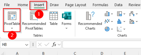
➤ First, click anywhere inside the dataset and go to the Insert tab from the top menu bar.
➤ Now, click on PivotTable in the Tables group. A new pop-up will appear.
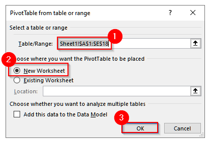
➤ In that window, select New Worksheet and click OK.
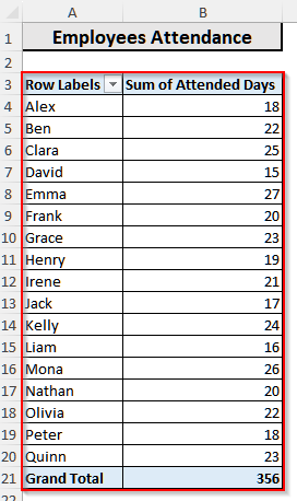
➤ Go to the PivotTable Fields pane, drag Employee Name into the Rows area, and drag Attended Days into the Values area.
➤ Now, you will see the pivot table is ready. Click anywhere on the Pivot Table to open the PivotTable Analyze tab.
➤ Then, select the PivotTable Analyze tab. You will see a group called Calculations. Select Fields, Items & Sets from that group.
➤ A new list of options will appear. Choose Calculated Field from that list. Another window will pop out.
➤ Now, in the Name dialog box of that new pop-up, type Attended >20 Days.
➤ Then, in the Formula box, enter the following formula:
=IF(Attended Days>20,1,0).
➤ Click Add and then OK.
➤ After that, click on cell E3 and write No of Employees Attended Office More Than 20 Days.
➤ Now, select cell E4 and insert the following formula:
=COUNTIF(C4:C20,1)
➤ Press Enter, and you will see the total count of employees who attended more than 20 days in the month.

Steps to Use COUNTIF Function in Pivot Table with Calculated Field
Though pivot tables are a great tool for summarizing and analyzing large datasets, they do not allow us to apply customized conditions directly. So, to cope with this, we can use the COUNTIF function with helper columns and achieve the desired outcome.
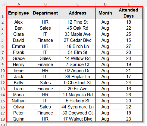
We will use the dataset below to explain how you can use the COUNTIF function with a helper column in Excel.
Step 1: Create a Pivot Table from the Dataset
First, we need to create a pivot table from our dataset.
Steps:
➤ First, click anywhere inside the dataset.
➤ Then, go to the Insert tab from the top menu bar.
➤ Now, click on PivotTable in the Tables group. A new pop-up will appear.
➤ In that window, select New Worksheet to place the pivot table.
➤ Finally, click OK, and a blank pivot table will appear in the new worksheet.
Step 2: Set Up the Pivot Table Fields
Now, we will set up the blank pivot table to analyze our dataset.
Steps:
➤ First, go to the PivotTable Fields pane and drag Employee Name into the Rows area.
➤ Then, drag Attended Days into the Values area. By default, it will show the Sum of Attended Days.
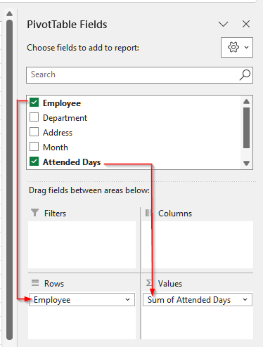
➤ Now, you will see the pivot table is ready.
Step 3: Add a Calculated Field
After creating the pivot table, we will add a calculated field to our pivot table to find the employees who have attended the office in August for more than 20 days.
Steps:
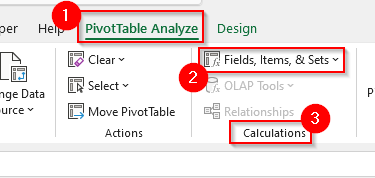
➤ First, click anywhere on the Pivot Table to open the PivotTable Analyze tab.
➤ Then, click on the PivotTable Analyze tab. You will see a group called Calculations. Select Fields, Items & Sets from that group.
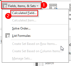
➤ A new list of options will appear. Choose Calculated Field from that list. Another window will pop out.
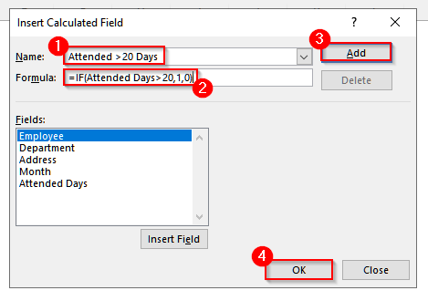
➤ Now, in the Name dialog box of that new pop-up, type Attended >20 Days.
➤ Then, in the Formula box, enter the following formula:
=IF(Attended Days>20,1,0)
➤ Click Add and then OK.
Step 4: Use the COUNTIF Function
Now, finally, we will use the COUNTIF function on the new field and get the total number of employees who came to the office more than 20 days, as well as those who did not.
Steps:
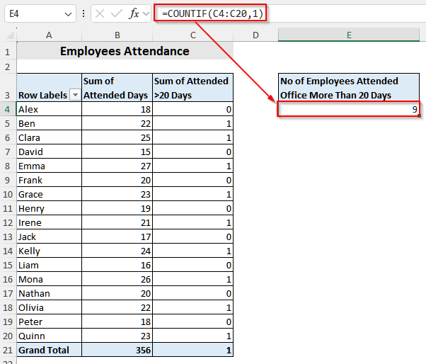
➤ First, click on an empty cell. For our data, we will click on cell E3 and write No of Employees Attended Office More Than 20 Days.
➤ Now, select cell E4 and insert the following formula:
=COUNTIF(C4:C20,1)
➤ Now, press Enter, and you will see the total count of employees who attended more than 20 days in the month.
Frequently Asked Questions
Can I use COUNTIF with three criteria in Excel?
No, you cannot use the COUNTIF function for three criteria. This function can only handle one criterion at a time because it is designed for single-condition counting. If you need to apply multiple conditions, you have to either combine multiple COUNTIF functions or use the COUNTIFS function. Suppose you have a few employees’ attendance in cells E2 to E18. Now, with the COUNTIF function, you can easily count employees who attended more than 20 days by using the following formula:
=COUNTIF(E2:E18,">20")
However, if you want to add more conditions, like department or month from your dataset, you’ll need COUNTIFS instead.
Can I Directly Perform Conditional Count in Pivot Tables?
No, you cannot. Pivot tables do not support logical conditions like greater than 20, etc., by default. These tables are designed to summarize data using basic operations such as sum, count, average, etc.. However, you can still perform conditional counting by using simple tricks. One way is to add a helper column in your dataset with an IF formula. Another option is to create a calculated field and use the COUNTIF function to get the conditional count.
Can I Get a Unique Count in a Pivot Table?
Yes, you can. To do this, you need to add your dataset to the Data Model while creating the pivot table. Once the pivot table is set up, place the field in the Values area, go to Value Field Settings, and select Distinct Count. This will give you the unique count instead of counting duplicates.
Wrapping Up
In this article, we learned how to use the COUNTIF function in a pivot table. The pivot tables do not support the use of the COUNTIF function directly on them. However, you can easily add a calculated column and use the COUNTIF function to apply a condition and get the count of things. Give it a try and let us know if you have any inquiries or any feedback.