Filtering and sorting are frequently used in pivot tables. Imagine you are a manager of a warehouse, you might want to see if you have high enough stock levels for the next month by checking if the stock is equal to or greater than the demand. In this tutorial, we will learn how to use pivot table filter values greater than in Excel.
➤ In the compact view, go to the Row Labels column, and click on the small sign at the right of the heading.
➤ Go to Value Filters > Greater Than.
➤ From the new dialog box, enter the value you want the output values to be greater than.
➤ Press OK.
If you don’t want to use the default filter option, there are other ways as well. In this article, we will go in-depth on how to filter values greater than a number in a pivot table. So, stick around and read the whole tutorial to learn more.
Filtering Values Using Greater Than Filter
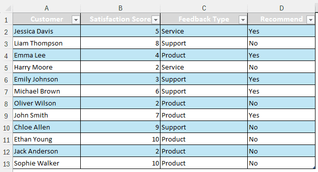
We have a feedback sheet about customer satisfaction here. The customers rated the product/service on a scale of 1-10. We want to filter out the customers who have given satisfaction ratings over 5.
Here’s how we do that:
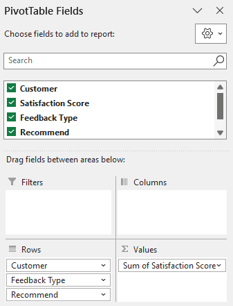
➤ After creating the pivot table, make sure that all the fields are selected from the PivotTable Fields panel.
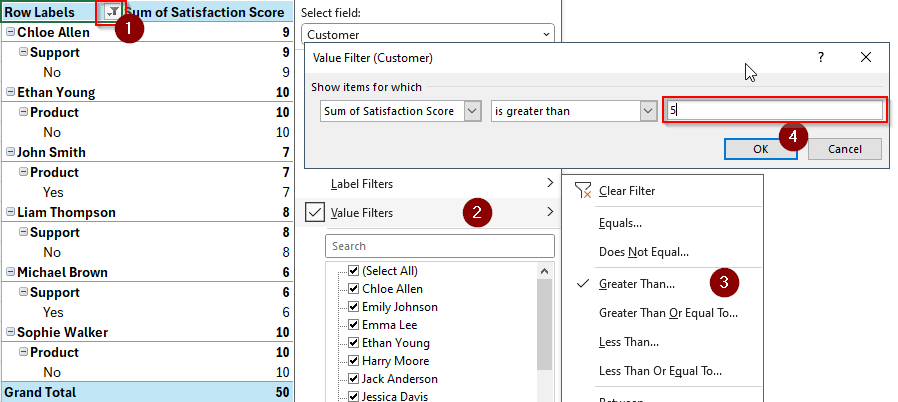
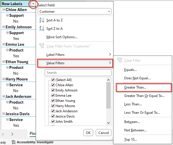
➤ From the “Row Labels” column, click on the small arrow with the heading that points downwards. A context menu will open.
Note:
If you are using the Outline/Tabular layout, you need to go to the Customer column.
➤ Go to Value Filters and select Greater Than…
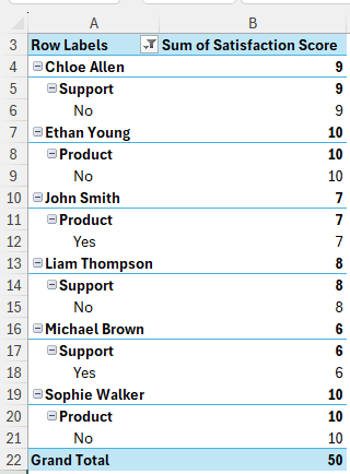
➤ In the new dialog box, write 5 as we want our values to be greater than 5. Change it according to your dataset. Press OK afterward.
➤ Now the pivot table will only show rows containing a value greater than 5.
Filtering Using a Helper Column
Instead of filtering the pivot table, we can change the source and add a helper column to filter out the values greater than 5. Follow the procedure below to do that:
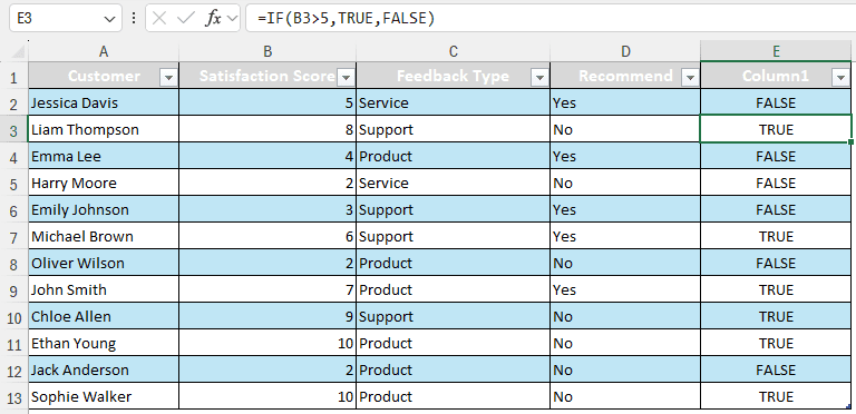
➤ Take a helper column to the right of the table, and write this formula:
=IF(B2>5,TRUE,FALSE)
➤ Upon pressing Enter, Excel will automatically fill the whole table with the filter values.
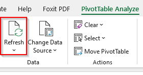
➤ Go back to the pivot table and refresh the table to make it aware of the changes in the source table. To do that, go to the PivotTable Analyze tab and hit Refresh.
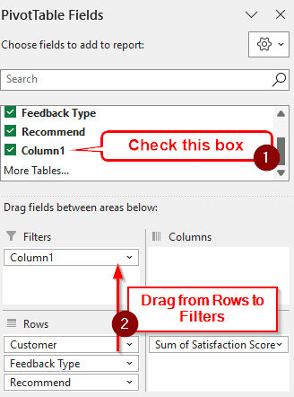
➤ Check the new Column1 box, and drag the field from the Rows area to the Filters area
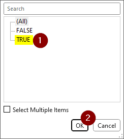
➤ From the pivot table, find the Column1 cell at the top (Usually at A1), and click the small arrow from the B1 cell.
➤ Select TRUE and hit OK.
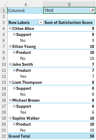
➤ Now the pivot table will be filtered with values greater than 5.
Frequently Asked Questions
How do you filter by value range in PivotTable?
First, make sure that the value range is checked in the pivot table fields panel on the right. Then, move the value range to the Filters area. The value filter will be available with the pivot table of the sheet. From the dropdown menu with the filter, select the value range and hit OK.
How to filter distinct count in pivot table?
While creating the pivot table, make sure that the table is added to the data model. After opening the PivotTable Fields panel, go to the Values area, and open the drop-down menu of your selected value. Select Value Field Settings, and select Distinct Count from the list of functions.
How do you filter greater than?
In a regular data range, you can filter greater than by going to the Home tab and clicking Sort & Filter. From there, create a filter. From the column heading, open the dropdown menu of the filter, and go to Number Filters > Greater Than. You can filter the data from the new dialog box.
How do you count highest to lowest in a PivotTable?
Right-click on the cell that you want to count from highest to lowest in the pivot table. Head to Sort > Sort Largest to Smallest, and your data would be sorted from highest to lowest.
How to pivot a table in Excel?
Make sure your data is in a table format. Click on any cell of the table, and go to the Table Design tab. From the Tools section, select Summarize with PivotTable. A new dialog box will open with options from which you can create a pivot table.
Wrapping Up
In this article, we learned how to use the pivot table filter values greater than in Excel. We hope that you will be able to adopt and use these two methods for your dataset. Download the spreadsheet used in this article so that you can follow the exact steps we did for your practice. Leave your suggestions below and let us know what other tutorials you want from us in the future.