Pivot Tables are used for summarizing large datasets, but often, the summarized data needs to be pulled into a different sheet for analysis. Excel’s built-in GETPIVOTDATA function is designed to extract specific data from a Pivot Table. This function works well when you need to pull information from a Pivot Table into a different worksheet.
In this article, we will guide you through three methods for using GETPIVOTDATA to pull values from a separate sheet, ranging from simple direct referencing to dynamic extraction across multiple tables.
To use GETPIVOTDATA from another sheet in Excel, here is one simple solution by using the GETPIVOTDATA function in Excel.
➤ Choose a cell in another sheet, write down the formula below:
=GETPIVOTDATA(“Total Price”,Pivot_Jan!$A$3,”Category”,”Bakery”,”Region”,”East”)
➤ Press ENTER, and you will get the result extracting data from Pivot Table in another sheet.

Overview of the Excel GETPIVOTDATA Function
The GETPIVOTDATA function in Excel is used to extract specific data from a Pivot Table. Instead of manually referencing cells, it retrieves values from the Pivot Table based on field names and item names. It also ensures the results remain accurate even if the Pivot Table layout changes.
Syntax
=GETPIVOTDATA(data_field, pivot_table, [field1, item1], [field2, item2], …)
| Argument | Description |
|---|---|
| data_field | The name of the Pivot Table data field you want to retrieve (e.g., “Total Sales”). Must be enclosed in quotes. |
| pivot_table | A reference to any cell in the Pivot Table. Excel uses this to identify which Pivot Table to pull data from. |
| [field1, item1] | (Optional) The field and item pairs specify which part of the data you want. You can include multiple field/item pairs. |
Applying GETPIVOTDATA Function to Extract Specific Data from Another Sheet
Using the GETPIVOTDATA function, you can extract specific data from a Pivot Table based on multiple criteria. The data will remain the same even if the field list changes in the Pivot Table.
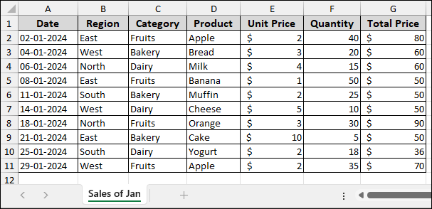
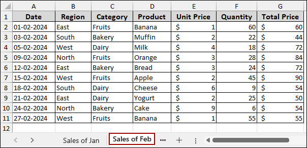
Imagine we have a sample dataset containing sales records with columns for Date, Region, Category, Product, Unit Price, Quantity, and Total Price. This data is placed in the “Sales of Jan” sheet.
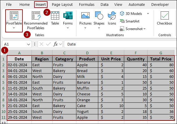
Now, we will create a Pivot Table with this data.
➤ Select the dataset, go to the Insert tab, and click PivotTable.
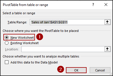
➤ In the dialog box, select New Worksheet and click OK.
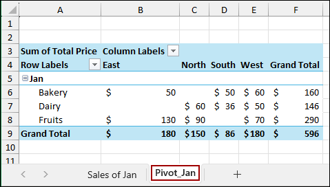
In the resulting Pivot Table, we have placed Region in the Columns area, Category in the Rows area, and Sum of Total Price in the Values area. The new sheet is named Pivot_Jan.
Now, we will extract the sales of Bakery items from the East region to a separate sheet named “All Sales“.
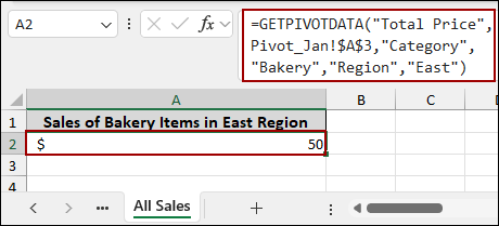
➤ In the “All Sales” sheet, choose cell A2, type the formula, and press ENTER.
=GETPIVOTDATA("Total Price",Pivot_Jan!$A$3,"Category","Bakery","Region","East")
This formula uses the data_field (“Total Price”), the pivot_table (defined by cell Pivot_Jan!A3), and two pairs of field/item arguments: (“Category”, “Bakery”) and (“Region”, “East”).
As a result, we will successfully retrieve $50 by pulling data from a PivotTable using the GETPIVOTDATA function.
Using GETPIVOTDATA Function to Pull Data Using Cell References
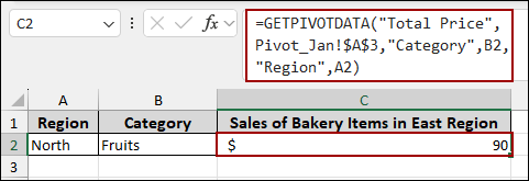
Editing formulas can limit uses and lead to errors. To prevent errors, you can replace these values with cell references. This will allow you to change the region or category easily without editing the formula itself. Here, we have set up two input cells: one for Region (A2) and one for Category (B2).
➤ In cell C2, enter the formula and Press ENTER.
=GETPIVOTDATA("Total Price",Pivot_Jan!$A$3,"Category",B2,"Region",A2)
In this formula, we replaced the item criteria with cell references: B2 for Category and A2 for Region.
As the Region is set to “North” (A2) and Category is set to “Fruits” (B2), the formula correctly returns $90, pulling the specific value from the Pivot Table.
Combining GETPIVOTDATA and INDIRECT Functions to Collect Data from Multiple Pivot Tables
For more advanced reporting, you might need to pull data from multiple Pivot Tables across different sheets. In that case, you can use the combination of the GETPIVOTDATA and INDIRECT functions to collect data.
Imagine a second dataset containing sales records for February, named “Sales of Feb”.
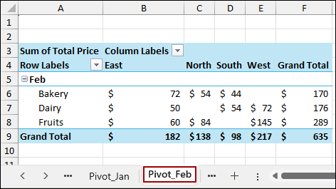
Following the previous methods, we will create a Pivot Table with the sample data and name it Pivot_Feb. The structure of the Pivot_Feb table is identical to Pivot_Jan.
To switch between the two Pivot Tables dynamically, we will use Data Validation to create a dropdown list of sheet names (months).
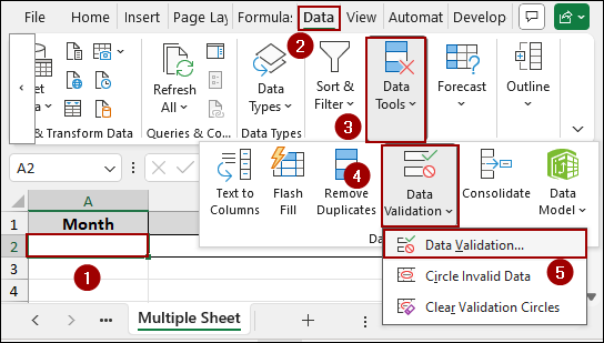
➤ In a new sheet named “Multiple Sheet“, select cell A2.
➤ Go to the Data tab, click on Data Tools, and select Data Validation.
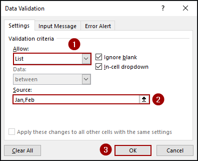
➤ In the Data Validation dialog box, select List for the Allow criteria.
➤ In the Source field, type the names of the Pivot Table sheet Jan,Feb.
➤ Click OK.
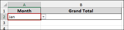
Thus, the cell A2 will get a dropdown menu allowing for the selection of Jan or Feb.
➤ Simply, select Jan from the drop-down list.
Now we will write the formula to dynamically change the sheet reference based on the month selected in cell A2. Here, we will extract the Grand Total from the respective Pivot Table.
➤ In cell B2, enter the following formula and hit ENTER.
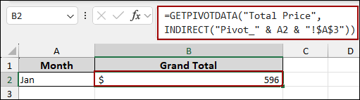
=GETPIVOTDATA("Total Price",INDIRECT("Pivot_" & A2 & "!$A$3"))
➥ The string "Pivot_" is concatenated (&) with the value in cell A2 (e.g., "Jan"). This creates the sheet name string to "Pivot_Jan".
Finally, we can add the Pivot Table’s top-left cell: “Pivot_Jan!$A$3”. Here, the INDIRECT function turns this text into a true reference, allowing the GETPIVOTDATA function to successfully pull the Grand Total.
As a result, with Jan selected in A2, the formula returns the correct Grand Total: $596.
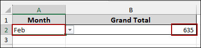
If the selection in cell A2 is changed to Feb, the formula automatically updates the Pivot Table reference to Pivot_Feb and returns the new Grand Total of $635.
Frequently Asked Questions
Can I use GETPIVOTDATA if the Pivot Table structure changes?
Yes. The data_field argument and the field/item arguments will always work regardless of where those fields are placed (Rows, Columns, or Filters). However, if you change the cell defining the Pivot Table’s top-left corner, you must update the formula.
How can I stop Excel from automatically generating GETPIVOTDATA when I click on a Pivot Table cell?
Excel automatically inserts the formula when you type equal (=) in another cell and click a value inside a Pivot Table. To disable this feature, go to the PivotTable Analyze tab. In the PivotTable group, click the Options drop-down arrow and uncheck the option Generate GetPivotData.
Does the GETPIVOTDATA function work with Pivot Charts?
No. The GETPIVOTDATA function only works by referencing a specific cell within a Pivot Table. It cannot directly extract data from a Pivot Chart. You must point the formula to the underlying Pivot Table on the sheet.
Concluding Words
Above, we have explored three methods to use GETPIVOTDATA from another sheet in Excel. The GETPIVOTDATA function is helpful, but its true utility shines when combined with sheet references and the INDIRECT function. Using the above methods, you can easily extract a fixed value, build a dynamic report using cell references, or pull data from multiple sheets. If you have any questions, please don’t hesitate to share them in the comments section below.