Grouping date fields is one of the features of Excel Pivot Tables, allowing you to instantly summarize daily transactions by months and years. This feature turns data into meaningful time-based reports, like monthly or annual sales summaries. Modern versions of Excel (2016 and newer) often group dates automatically when you drag the Date field into the Rows area. However, if this automatic grouping doesn’t happen, you might need to group dates manually.
In this article, we will guide you through two methods to group dates by month and year in Excel Pivot Table.
To group dates by month and year in Excel Pivot Table, here is one simple solution by dragging the dates.
➤ Ensure your source data’s date column is formatted as a Date (not Text).
➤ Drag the Date field into the Rows area, and Excel will create separate fields for years and months.
Dragging Dates into Pivot Table Field for Grouping by Month & Year
In the latest versions of Excel, the easiest way to group dates is simply by dragging the date field into the Pivot Table areas. Excel automatically detects the date format and creates a group for months and years.
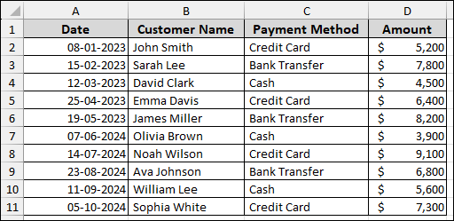
Imagine a sample dataset showing daily sales transactions. Here, we will create the Pivot Table and then drag the Date field into the Rows area.
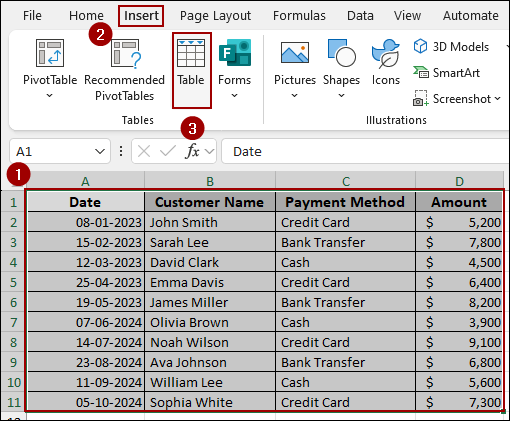
First, convert your raw data into a Table.
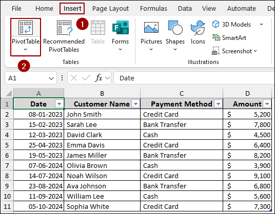
➤ Select the dataset (A1:D11).
➤ Go to the Insert tab, click Table.
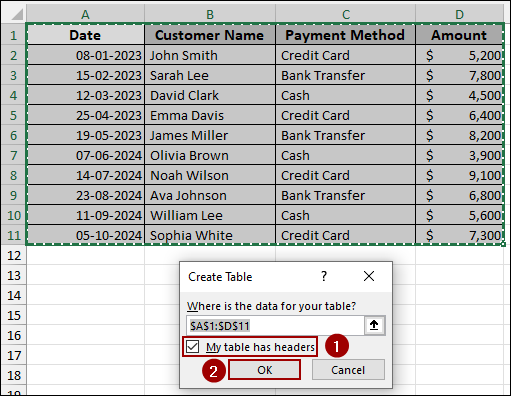
➤ Checkmark My table has headers and click OK.
Now, let’s insert the Pivot Table.
➤ Go to the Insert tab, click PivotTable.
➤ Select New Worksheet, and click OK.
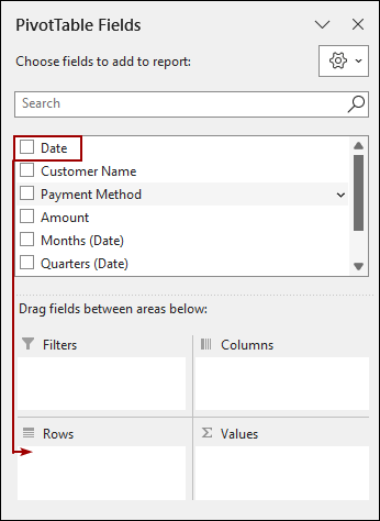
When you drag the Date field into the Pivot Table, Excel automatically groups it into a hierarchy.
➤ Drag the Date field into the Rows area.
Upon dragging the Date field, Excel automatically adds Years (Date), Quarters (Date), Months (Date), and the original Date field into the Rows area.
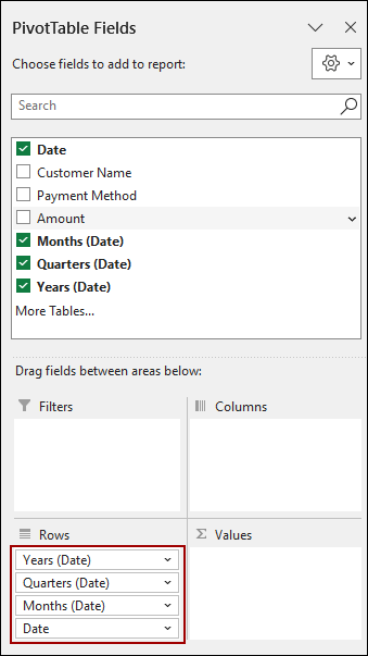
To group only by month and year, we need to remove the unwanted group fields (like Quarters and the original Date field).
➤ From the Rows area of the PivotTable Fields pane, click the dropdown for Quarters (Date).
➤ Select Remove Field.
➤ Repeat this step for the original Date field.
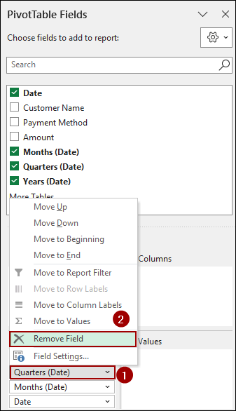
The final setup in the Rows area should contain only Years (Date) and Months (Date).
➤ Drag the Amount field into the Values area.
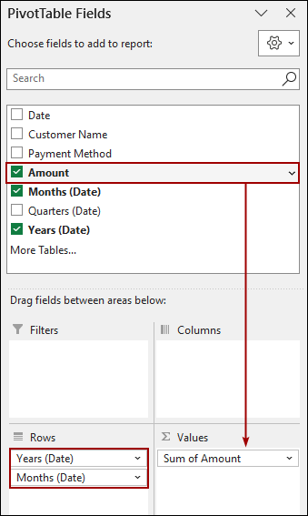
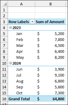
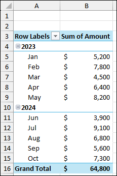
As a result, we have successfully grouped date by month and year, summarizing by Year (2023, 2024) with a list for each Month.

Note:
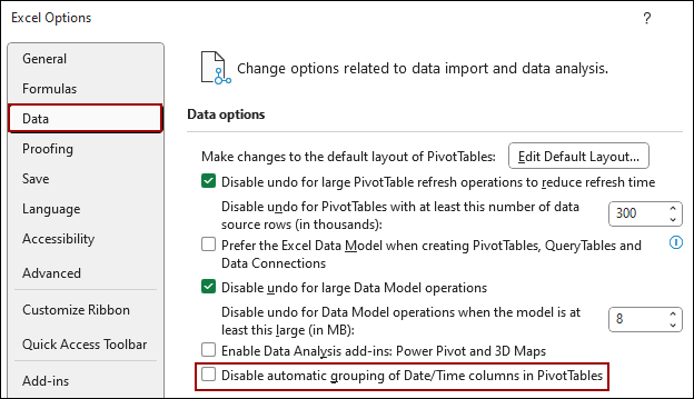
If you find that dragging the Date field does not auto-group, it may be disabled in your Excel options. You can re-enable it by going to File > Options > Data and unchecking Disable automatic grouping of Date/Time columns in PivotTables.
Using Group Selection Feature to Group Pivot Table Data
If your date field did not auto-group or you simply prefer the manual method, you can use the Group Selection feature in Excel.
If auto-grouping is disabled, your initial Pivot Table will list every transaction date individually. Here, we will use the same Pivot Table.
➤ Drag the Date field to the Rows area.
➤ Drag the Amount field to the Values area.
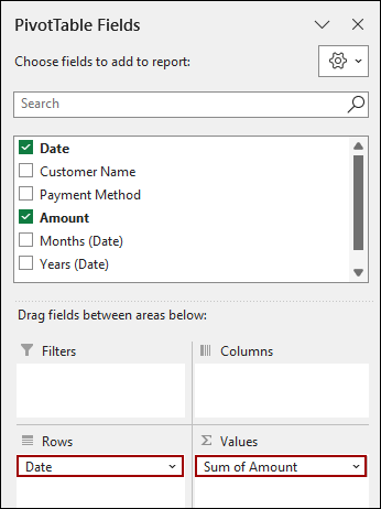
Your Pivot Table shows every single date from the source data. To group dates manually.
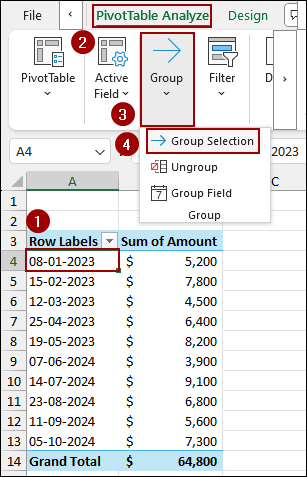
➤ Select any date from the list and click PivotTable Analyze > Group > Group Selection.
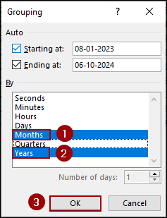
The Grouping dialog box will appear.
➤ Choose Month and Year from the By section and click OK.
The Pivot Table will group dates by the selected intervals, showing the sales summarized by year and month.
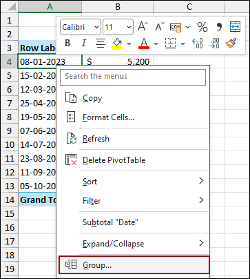
You can also use the context menu to group dates. For this,
➤ Right-click on any date cell in the Pivot Table.
➤ From the context menu, select Group.
➤ Select both Months and Years from the By list and hit OK.
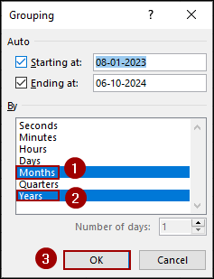
Finally, we have successfully grouped dates by month and year in Excel Pivot Table.

Frequently Asked Questions
Why is the Group option greyed out in my PivotTable?
This usually happens when the date field contains blank cells, text values, or errors. Make sure your column has only valid date values.
Can I ungroup dates after grouping them?
Yes. Right-click on the grouped field and choose Ungroup. This will return your PivotTable to individual daily dates.
Is it possible to group by a custom period, like every 7 days or every 2 months?
Yes. In the Grouping dialog, you can specify a custom Number of days (e.g., 7 for weekly grouping). For 2-month or 3-month intervals, you will need to use calculated helper columns before creating the PivotTable.
Concluding Words
Above, we have covered the two most effective methods for grouping dates in an Excel Pivot Table. For modern Excel users, the Drag and Drop method often works instantly by auto-creating the date hierarchy. For older versions, the Group Selection feature allows you to manually specify the exact time periods in days, months, quarters, or years. If you have any questions, please don’t hesitate to share them in the comments section below.