In a pivot table, slicers can be used to filter data easily. Slicers include the possible values of a column so that when you select a value, you only see the related fields in the pivot table. But when you have a lot of rows in your pivot table, the slicer becomes big, and it makes the worksheet hard to look at.
While using a dropdown filter in a regular table is easy and does not need a slicer, it is not the same for pivot tables. In a pivot table, if we use a filter, that field has to be removed from the pivot table and kept in the filters section. In order to eliminate this downside, we can create a dropdown from the slicer in Excel, and this article will show you how to do it.
➤ Create a slicer for the pivot table.
➤ Copy the pivot table to another location in the same sheet.
➤ Remove every other field other than the field you want to filter in the new pivot table, and move that field to the Filters section.
➤ Use the new pivot table as the dropdown slicer.
Slicers don’t support the dropdown function, so we have to improvise and be creative with our solution. In this article, we will create a dropdown for our pivot table that will use a slicer in the background to filter the table.
Steps for Creating a Dropdown Slicer in Excel
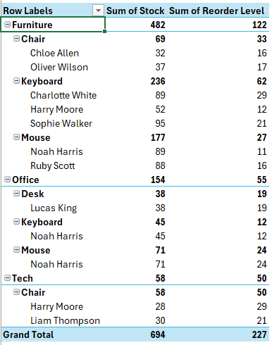
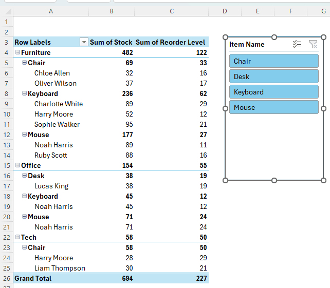
Slicers cannot be directly converted to a dropdown, but we can mimic the function in other ways. Before demonstrating the steps, let’s take a look at the dataset. We have created a pivot table from some data on office supplies. There are item names, the categories of those items, stock and reorder levels, and supplier names. We will add a slicer and make a dropdown menu using the slicer. Let’s begin:
Step 1: Add a Slicer
First, let’s add a slicer to the pivot table like we do in general. Then, we will make a dropdown using it:
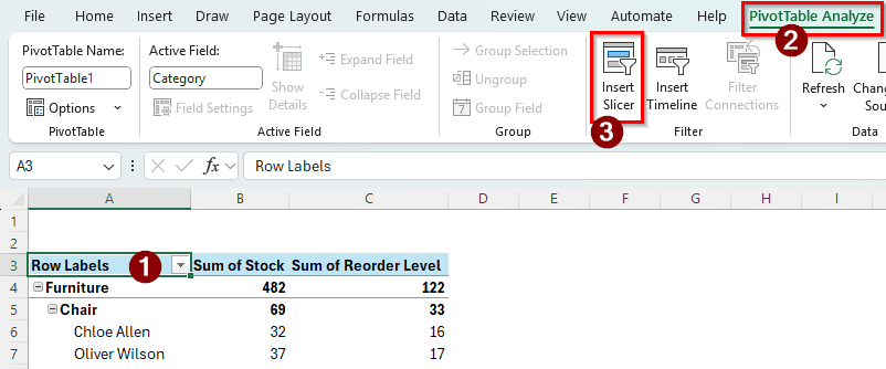
➤ Click on a cell of the pivot table to enable the related tabs in the Excel ribbon.
➤ Go to the PivotTable Analyze tab, and find the Filter group.
➤ Click on the icon that says “Insert Slicer”.
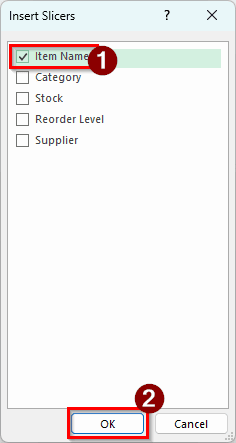
➤ Select “Item Name” and press OK to add a slicer for the Item Name column.
➤ The slicer should be visible in the worksheet now.
Step 2: Copy and Customize the Pivot Table
We need to copy the existing pivot table to create a new one that has a connection with the existing slicer. It will help us create a dropdown filter. Follow the instructions below, don’t just copy and paste the pivot table like you usually do.
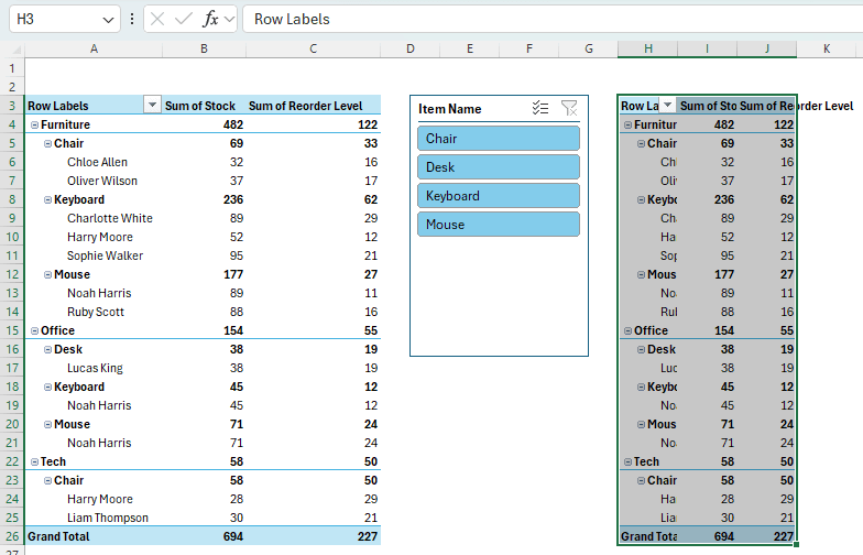
➤ Select the pivot table (Range of A3:C26).
➤ Press Ctrl + C to copy the table.
➤ Go to H3 and press Enter to paste the table.
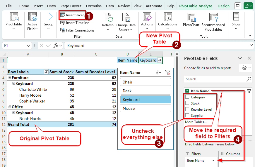
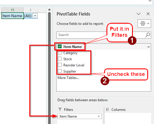
➤ Move Item Name to the Filters section in the new pivot table.
➤ Uncheck all the other fields of that pivot table as well.
Step 3: Finish Creating the Dropdown
Most of the work is done; we just need to make the dropdown look like one and use it for our purposes. Here is what we have to do:
➤ Move the pivot table to the range of D1:E1. The pivot table is only two cells (H1:I1) now, so it should not require any more space.
➤ Select H1:I1 and press Ctrl + X to cut the table.
➤ Press Enter on the D1 cell to paste the table there.

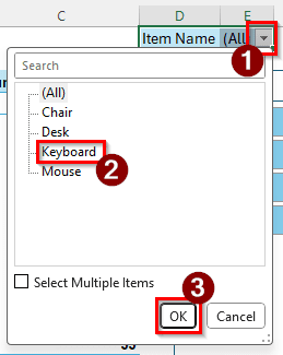
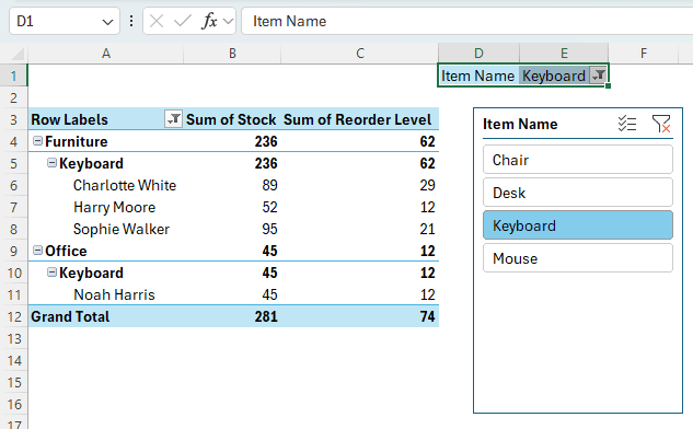
➤ Now select your desired filter from the dropdown in E1 to use the slicer. The slicer will update as you select the filter.
➤ For example, we can select Keyboard to filter the data using the Keyboard filter.
➤ The slicer has been updated for the pivot table, and the pivot table has been sorted.
Frequently Asked Questions
How do I add a drop-down filter in Excel?
You can do this by two methods in general. The generic way to select the data range and go to the Editing group. Then select Sort & Filter > Filter from the Home tab to add a drop-down menu in the column headers. The second method is to just convert the range to a table. Select the data range, and press Ctrl + T to create a table. You can also change the range in the small tool window that pops up. Press OK to confirm and see the table and filter in action.
How to get the slicer option in Excel?
To add a slicer in a regular table or data range, go to the Insert tab in the ribbon and select Slicer from the Filters group. A new window will pop up for creating the slicer. However, your dataset must be connected to a data model to use the slicer.
How to set up a drop-down in Excel?
Go to the cell where you want the drop-down to be, and find the Data tab. From the Data Tools group, open Data Validation, and select Data Validation again from the dropdown. Set up the validation criteria and the cells from the new window, and press OK to create the dropdown.
How to create a drop-down list in Google Sheets?
In the target cell, enter @ and select Dropdowns from the components. You can also add it by going to the Insert menu and selecting Dropdown. Then, change/add items to the dropdown from the data validation rules panel.
What is a dropdown menu?
A dropdown menu is a type of menu that does not take up a lot of space but allows the user to select an option from a list when clicked. In Excel, dropdown menus are used for data validation and selecting fields from a list.
Wrapping Up
In this article, we have learned how to create a dropdown menu from a slicer in an Excel pivot table. Leave what topic you want our next tutorial to be on. Download the Excel file we used in this article to see the dropdown slicer in action and have a real example on your hands. Stay tuned, and we will see you in another article.