In a table with a large dataset, it is often hard to determine which values are larger or smaller than the others. If you have a worksheet with sales data, you might want to see the top performers at a glance. In Microsoft Excel, it is very straightforward to sort the data from largest to smallest and vice versa. In pivot tables, although it works differently from a regular dataset, it is much easier to sort while keeping the data intact. In this article, we will show you a step-by-step guide on how to sort a pivot table from largest to smallest.
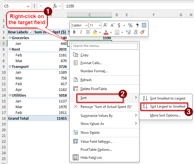
➤ Right-click on the field that you want to sort.
➤ Go to Sort > Sort Largest to Smallest
Pivot tables sort according to different rows, and it can be confusing at first glance. But when you are working with pivot tables, you expect it to show up like one. For a proper example and demonstration on how to do the sorting, read the full tutorial.
Sorting Pivot Table from Largest to Smallest
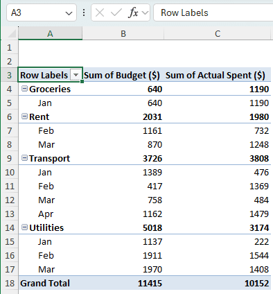
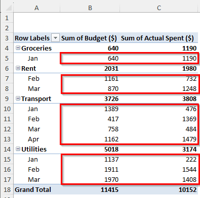
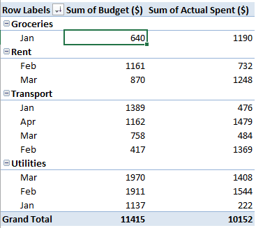
We have a dataset here with some financial data. There are the budgets for each category and month, and there are the amounts that were actually spent. We want to sort it from largest to smallest to know the largest budget amounts that were set against the spent amount. Follow the steps below to sort the pivot table:
Step 1: Decide the Field and Method
As a pivot table sorts only by the fields, you cannot just randomly select a cell and ask it to sort. That way, the sorting won’t be what you want. Here is what you need to do:
➤ If you need to sort the values by categories, you need to select a subtotal cell. Selecting B4/C4 or B6/C6 or B9/C9 or B14/C14 will work.
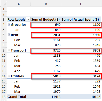
➤ This will not sort the values inside the Month field. Only the Category types will be sorted.
➤ If you want to sort the values inside the month, select any cell inside the month field. You can select one from B5:C5, B7:C8, B10:B13, and B15:B17.
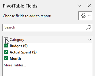
➤ If you want to sort not by the categories, but the values for the months, remove the Category field from the Rows by unchecking it from PivotTable Fields. However, we will not do that for this tutorial.
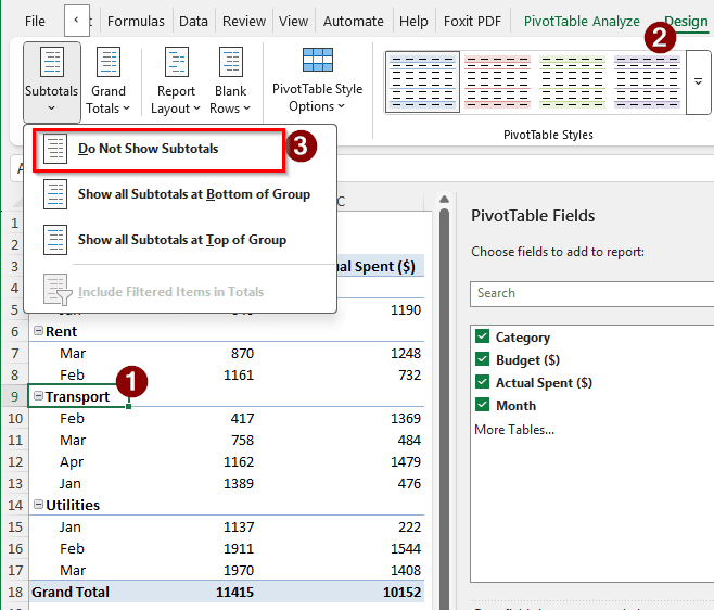
➤ The subtotals for each category might break the illusion of sorting. You can turn them off by selecting any cell of the pivot table, then going to the Design tab of the Ribbon. Find the Layout section, and hit Do Not Show Subtotals from the Subtotals button.
Step 2: Sort the Pivot Table
There are essentially two places from which you can access the sort functions. Follow the instructions below:
➤ The first method is from the Ribbon of Microsoft Excel. From the Ribbon at the top of the Excel window, find the Data tab, and locate Sort & Filter. Make sure you have the target cell selected.
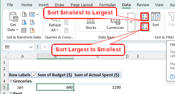
➤ There are three buttons in the left section. Hit the Sort Largest to Smallest button to sort it.
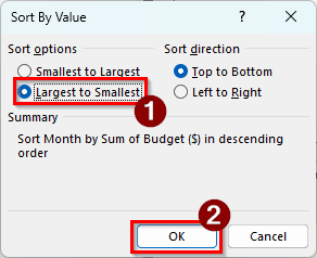
➤ You can also click the Sort button directly to choose advanced sorting options like below. Select the options you like and press OK afterwards. We are selecting Largest to Smallest and pressing OK for this example.
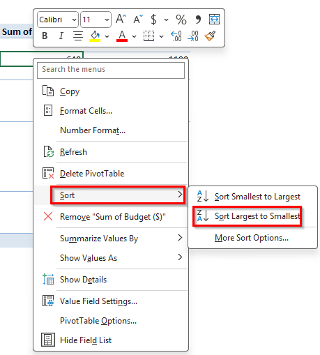
➤ The second choice is to right-click on the field to open the context menu that has a lot of options, including sorting.
➤ Go to Sort > Sort Largest to Smallest to commit the sorting.
➤ You can also select More Sort Options to open the window from before that allows you to sort by value.
Frequently Asked Questions
How to make a PivotTable in Excel bigger?
You can add more data in the source table, and refresh the pivot table afterwards to make the pivot table bigger. If you want it to be visually bigger, find the zoom slider on the bottom right of Microsoft Excel. It should be 100% by default. You can move the slider to the right to make the table bigger.
How to sort a pivot table from largest to smallest in Google Sheets?
Click on a cell of the pivot table to open up the pivot table editor. On the values section, locate the field that you need to sort. There should be a dropdown arrow right next to the name of the field. Click on that, and select Sort by. Then, click on Z → A to sort from largest to smallest.
How to reorder PivotTable columns?
Right-click on the column that you want to reorder. From the context menu that pops up from the right-click, select Move. A submenu should appear, and you can select where you want to move the column from there.
How to show the top 10 in a pivot table?
Right-click on the field that you want to show the top 10 of. From the context menu, select Filter > Top 10. In the new window, there will be four fields to fill out. Keep the first two intact, and change the last two according to your requirements.
How do you reorder rows in a pivot table?
There are two ways to do this. To reorder the whole field, you can drag the row headings that show up in the Rows section of the PivotTable Fields. If you want to move the individual entries in the rows, you can right-click on them and go to Move to move them to preferred locations.
Wrapping Up
In this tutorial, we have learned how to sort a pivot table from largest to smallest. The next time you find yourself in a position where you have to sort a pivot table, you know how to do it already. The Excel file where we followed the steps we have provided here is available for you to download. In case you have any questions regarding this article or Excel in general, leave them in the comment section, and we will get back to you.