Displaying text from another cell in Excel is a common task for data analysis and for automating your workflow. Whether you are creating summaries, performing complex lookups, or simply reformatting data, referencing another cell is an essential technique. For example, you have dates in your data in a given format, but you want to display them in another format. You can easily do this in Excel. This article covers 8 easy methods to achieve this, from the simplest direct referencing to powerful lookup formulas and conditional logic.
➤ Go to the cell where you want to display text from another cell.
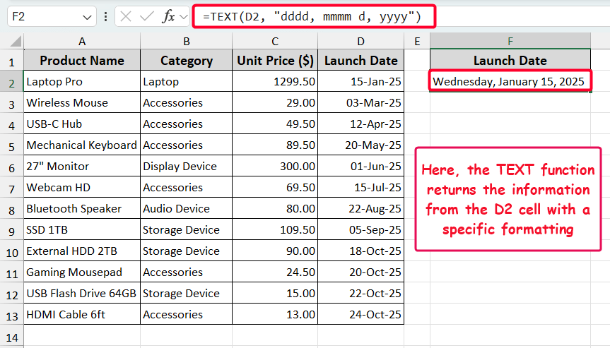
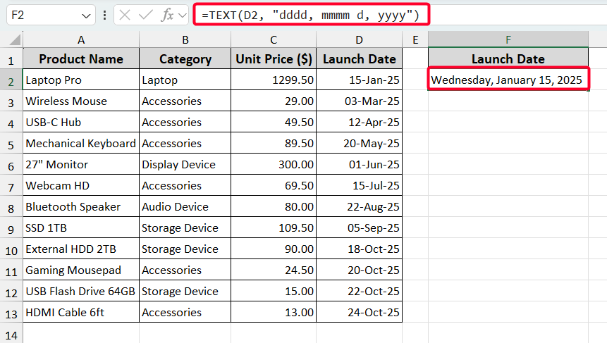
➤ Put the formula: =TEXT(D2, “dddd, mmmm d, yyyy”) in the F2 cell and press Enter.
➤ The TEXT function returns the date in a specified format, with the day name appearing first.
In this article, we will first show you a simple method, then show you how to display text with formatting and lookup conditions. Also, you’ll see how to extract a specific part of a text and pull a text from another sheet. Lastly, you’ll see how to use a named range and display text based on values with conditional logic.
Reference a Cell Directly with an Equal Sign
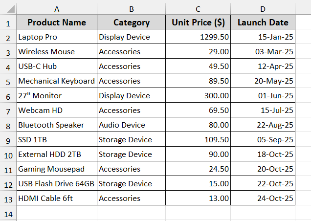
The simplest way to display text from another cell is by referencing the cell with an equal sign. Let’s have a look at the following dataset that will be used in this article. Here, we have a product inventory of 12 electronic products with category, unit price in dollars, and launch date.
Steps:
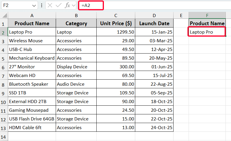
➤ Go to the F2 cell and enter the following formula.
=A2
➤ Press the Enter button to get the result.
Display Text From Another Cell Using TEXT Function with Formatting
When you need to format numbers, dates, or values as readable text strings, you can use the TEXT function. We have a date in date-month-year format, but we want to extract the date with full day-month-date-year format. Use the following formula.
=TEXT(D2, "dddd, mmmm d, yyyy")
Here, D2 is the source cell from which we want to extract. “dddd, mmmm d, yyyy” is the format code where “dddd” means full week day name, “mmmm” means full month name, “d” means day of month, and “yyyy” means 4-digit year.
Use VLOOKUP Function
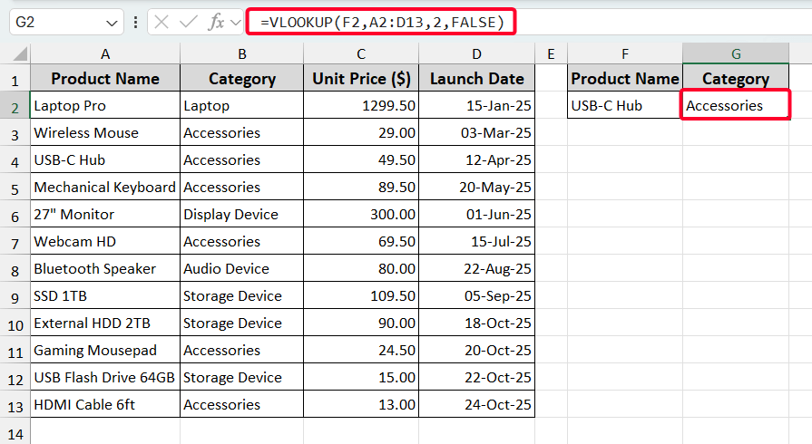
The VLOOKUP function helps you quickly find and return text from a table based on a lookup value. But it’s limited to rightward searches only. Now we want to extract the category name if the product name matches, which means we want to display the category “USB-C Hub” product name. To do this, use the following formula.
=VLOOKUP(F2,A2:D13,2,FALSE)
Here, F2 is the lookup value, A2:D13 is the lookup table from where we extract the data, 2 is the column index number as we want to find the category, and FALSE is for an exact match value.
Use INDEX-MATCH Formula
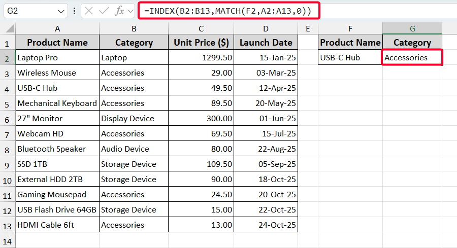
You can also use the INDEX-MATCH formula which is more powerful than VLOOKUP. Because it can do leftward searches and update dynamically. The formula is:
=INDEX(B2:B13,MATCH(F2,A2:A13,0))
Here, the MATCH(F2, A2:A13, 0) finds the row number where the lookup value (F2) matches from A2:A13 cells (0 is for exact matching). Later, the INDEX function returns the value from that row in the B2:B13 cells to find the category.
Display Specific Portion of Text From Another Cell
Sometimes you need to extract a specific portion of text from a cell. We can use the LEFT, MID, and RIGHT functions to do this.
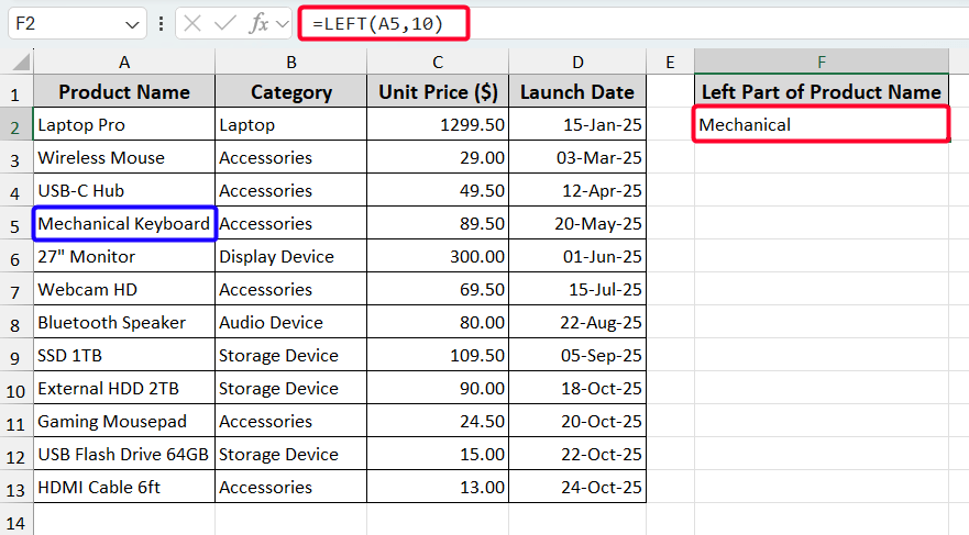
Extract Left Portion of Text
We want to extract the left portion (“Mechanical”) of the text, i.e., “Mechanical Keyboard”, available in the A5 cell. The formula will be as follows.
=LEFT(A5,10)
Here, 10 is the number of characters from the left.
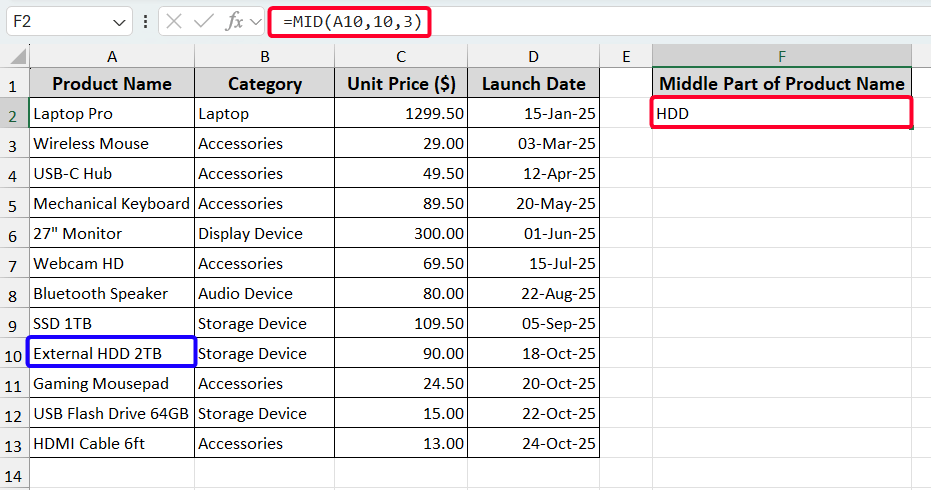
Extract Middle Portion of Text
Use the following formula to pull out the middle portion (“HDD”) of the text in the A10 cell (“External HDD 2TB”).
=MID(A10,10,3)
Here, 10 is the starting position and 3 is the number of characters to extract.
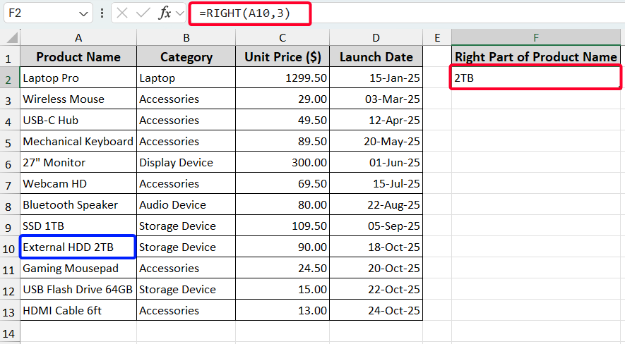
Extract Right Portion of Text
In case of extracting the right part (“2TB”) from the text (“External HDD 2TB”), use the following formula.
=RIGHT(A10,3)
Here, 3 means characters from the right.
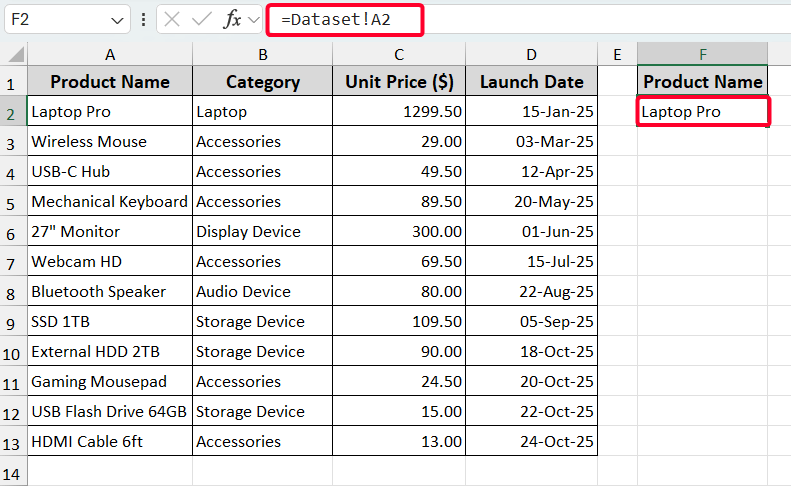
Display Text Another Sheet’s Cell
Pulling text from a different sheet keeps your main page clean. It syncs changes automatically until you don’t change the sheet name. For this, you have to just refer to the sheet name from where you want to extract the data. After adding the exclamation mark (!) after a sheet name, we can easily refer to a sheet. In the following formula, Dataset! is our source sheet.
=Dataset!A2
Display Text Using Named Range
A named range gives your cells friendly nicknames to make formulas shorter as well as to pull out the data easily.
Steps:
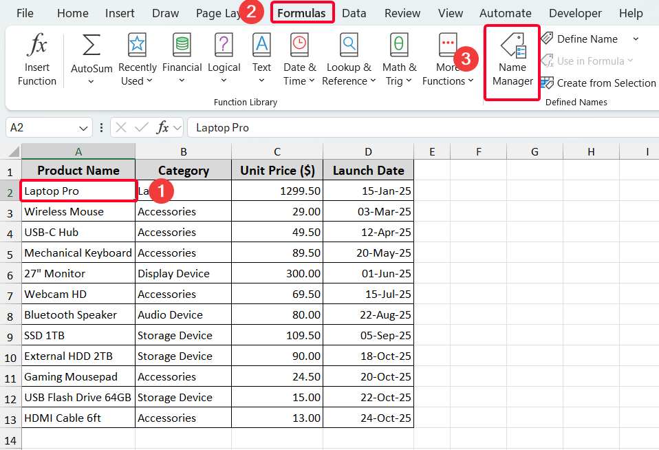
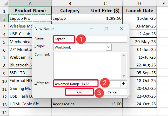
➤ First, select the cell that you want to enlist as a named range.
➤ Go to Formulas >> Name Manager.
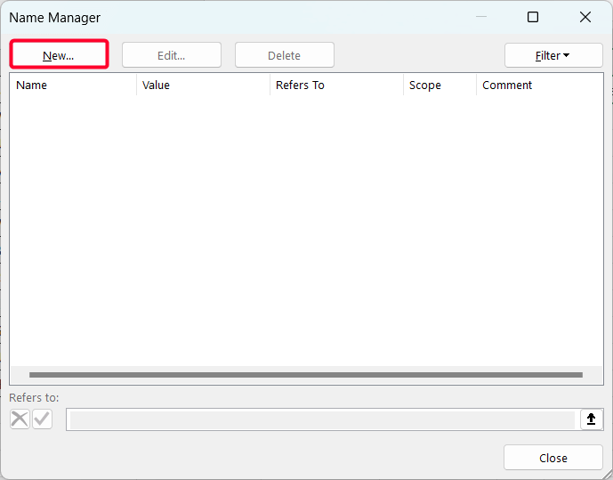
➤ Meanwhile, the Name Manager window will pop-up. Select the New option.
➤ Choose the name (e.g. Laptop).
➤ Check the Refer to option and press OK.
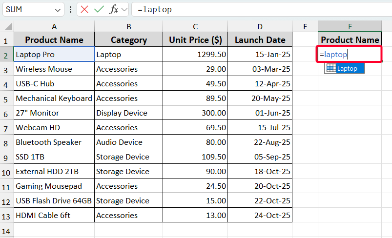
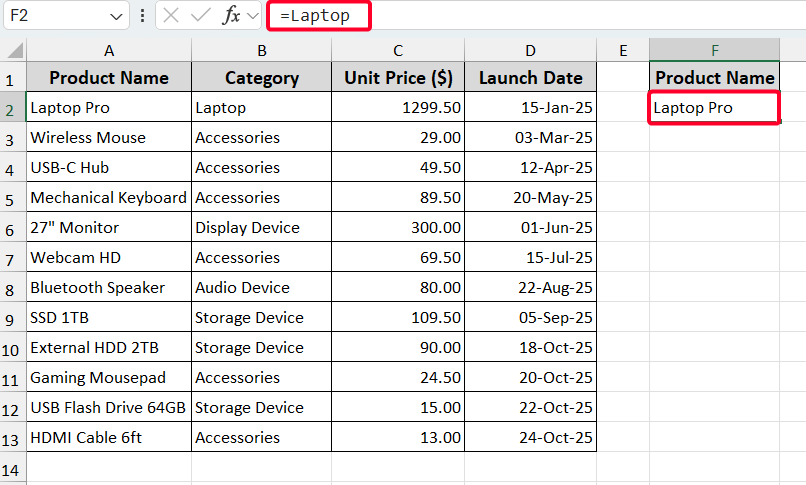
➤ Now, your named range is ready to pull out! Go to the F2 cell and type “laptop”. You’ll see it and select it.
Then you’ll get the product name.
Display Text Based on Values with Conditional Logic
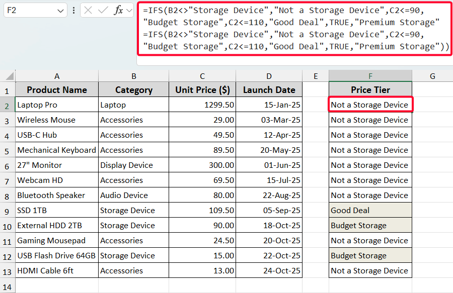
In some cases, you might need to display the text based on values and conditions if they meet. For example, we want to label the product name (category: storage device) as price tier: Budget Storage, Good Deal, and Premium Storage. We’ll use the IFS function to do this.
=IFS(B2<>"Storage Device","Not a Storage Device",C2<=90,"Budget Storage",C2<=110,"Good Deal",TRUE,"Premium Storage"
=IFS(B2<>"Storage Device","Not a Storage Device",C2<=90,"Budget Storage",C2<=110,"Good Deal",TRUE,"Premium Storage"))
Frequently Asked Questions
Can we combine text from multiple cells?
Yes, you can use the Ampersand (&) operator or the CONCAT/CONCATENATE functions to join text from different cells. For example, =A2 & ” – ” & B2 would combine the text from A2 and B2 with a dash.
What happens if we move the original cell?
If you use a direct cell reference (like =A2), Excel automatically updates the formula to the new location when you move the original cell.
How do we prevent the displayed text from updating when the original cell changes?
To make the text static, copy the cell containing the formula, then use Paste Special to paste only the values into the same or a new cell. This replaces the formula with the resulting text.
Are there common errors when displaying text from other cells?
Common errors include #REF! error due to invalid cell references. To get rid of this error, you have to be cautious when referencing a cell in the same sheet or a different sheet.
Wrapping Up
This is how you can easily display text from another cell in Excel. We have shown the method with a proper explanation. Download the practice workbook and practice hands-on. Share your issue if you face any trouble!