
Using the VLOOKUP function, you can compare two columns to determine if one column matches or not with the other column. To find matches or non-matches between two columns, the VLOOKUP function searches for a value in one column within another. In this article, we’ll explore various ways to compare two columns using the VLOOKUP function, from simple match tests to displaying common values and even returning actual data.
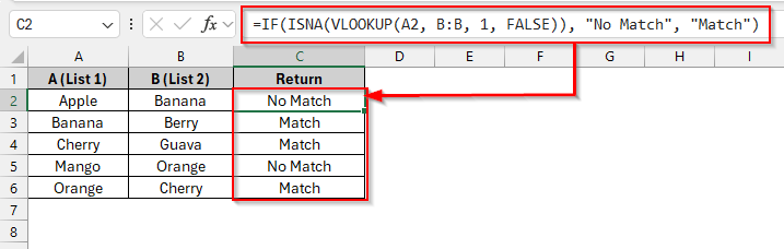
To compare two columns (Column A with Column B) using the VLOOKUP function, follow these steps:
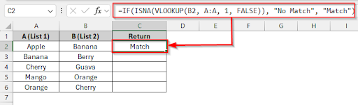
➤ Select the C2 cell.
➤ Write this formula in cell C2.
=IF(ISNA(VLOOKUP(A2, B:B, 1, FALSE)), “No Match”, “Match”)
➤ Press Enter, and you will see the matched and unmatched values in Column C
In this article, we will describe six methods about how to compare two columns in Excel using the VLOOKUP function. Identifying matches and Differences Between Two Columns, returning common Values, finding missing Values, comparing in Reverse, comparing two Columns in Different Excel Sheets, and returning a Value from the Third Column. These are the ways to compare two columns in Excel using the VLOOKUP function.
Identifying Matches and Differences Between Two Columns
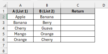
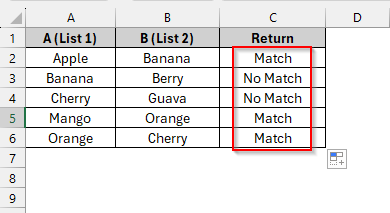
For this method, we’ll use a simple dataset of a fruit name list with two columns (Column A and Column B). The matched/non-matched values will be shown in column C by comparing the two columns.
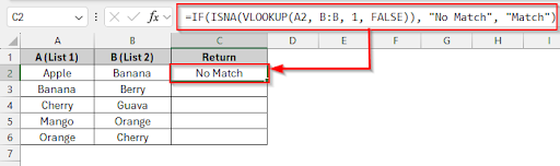
We’ll combine the IF, ISNA, and VLOOKUP functions. The VLOOKUP function searches for each value from Column A in Column B. If the value is found, the VLOOKUP function returns it; otherwise, it returns an error. Then, the ISNA function checks if there is a #N/A error. The IF function returns “Match” if the result is not an error; otherwise, it returns “No Match.”
Steps:
➤ Click on cell C2 and write this formula:
=IF(ISNA(VLOOKUP(A2, B:B, 1, FALSE)), "No Match", "Match")
➤ Press Enter and see the result in cell C2.
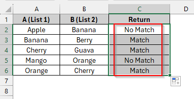
➤ Drag the formula down to see the result in other cells.
Returning Common Values
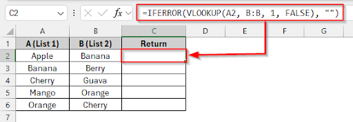
To return common values, we’ll combine the VLOOKUP function with the IFERROR function between two columns. The VLOOKUP function searches for each name from Column A within Column B. If a matched fruit name is found, it returns that fruit name; if not, it returns an error. The IFERROR function identifies the error and replaces it with a blank.
Steps:
➤ Click on cell C2 and write this formula:
=IFERROR(VLOOKUP(A2, B:B, 1, FALSE), "")
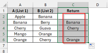
➤ Press Enter and see the result in cell C2. The result is blank because there is no actual matching value to return.
➤ Drag the formula down to see the actual matching value in other cells.
Finding Missing Values
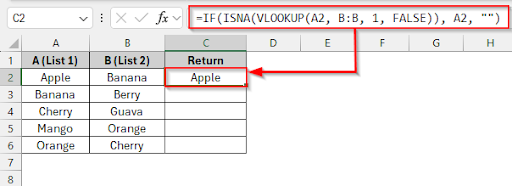
We’ll find the missing values after comparing Column A with Column B by using the VLOOKUP, ISNA, and IF functions. The VLOOKUP function searches for the value from Column A in Column B. If the value is not found, it returns an error. The ISNA function finds that error, and the IF function uses that error when it’s missing in Column B and shows that missing value; otherwise, it returns a blank.
Steps:
➤ Click on cell C2 and write this formula:
=IF(ISNA(VLOOKUP(A2, B:B, 1, FALSE)), A2, "")
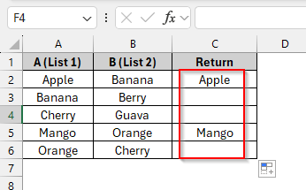
➤ Press Enter and see the missing value in cell C2.
➤ Drag the formula down to see the other non-matched/missing values in different cells.
Comparing in Reverse
In this method, we will compare the two columns in reverse, that means we’ll check Column B with Column A by using the VLOOKUP, ISNA, and IF functions. The VLOOKUP function searches for each value from Column B in Column A. If a matching value is found, it returns that value; otherwise, the ISNA function finds the error, and the IF function shows “Match” if the value is found or “No Match” if the value is not found.
Steps:
➤ Click on cell C2 and write this formula:
=IF(ISNA(VLOOKUP(B2, A:A, 1, FALSE)), "No Match", "Match")
➤ Press Enter and see the missing value in cell C2.
➤ Drag the formula down to see the reversed matched/non-matched values in different cells.
Comparing Two Columns in Different Excel Sheets
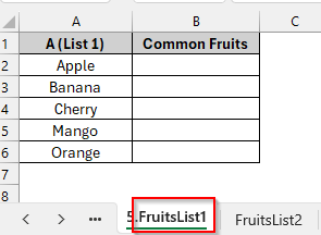
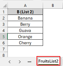
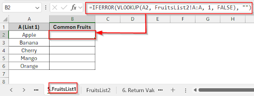
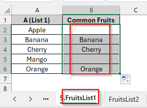
Now we have two columns which are located in different sheets. In the “FruitsList1” sheet, we have fruit names: Apple, Banana, Cherry, Mango, Orange, in Column A and in the other sheet, “FruitsList2”, we have fruit names: Banana, Berry, Guava, Orange, Cherry in Column A. We will compare those two columns using the VLOOKUP and IFERROR functions. Matched values will be returned from the “FruitsList2” sheet, and the unmatched values will be returned as blank.
Steps:
➤ In “ FruitsList1” sheet, click on cell B2 and write the formula:
=IFERROR(VLOOKUP(A2, 'FruitsList2'!B:B, 1, FALSE), "")
➤ Press Enter, and you will see the blank cell in cell B2 because there is no matching value “Apple” in the sheet “FruitsList2”.
➤ Drag down the formula to see the other matched values.
Returning a Value from the Third Column
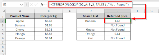
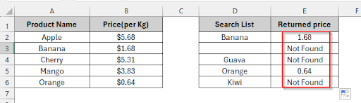
After comparing two columns, we will return a value from a third column by using the VLOOKUP and IFERROR functions. The VLOOKUP function searches each value from the 3rd column in Column A, and if a match is found, it returns the matched value from Column B. If no match is found, the IFERROR function finds the error and replaces it with “Not Found”.
Steps:
➤ Click on cell E2 and write this formula:
=IFERROR(VLOOKUP(D2, A:B, 2, FALSE), "Not Found")
➤ Press Enter and see the price for Banana, which is 1.68
➤ Drag down the formula to see the other values.
Frequently Asked Questions
What will be the result if a value is not found using the VLOOKUP function?
The VLOOKUP function returns a #N/A error if a value isn’t found after comparing two columns. Without showing the error, you can solve this problem by using IFERROR or ISNA functions to show custom messages or keep cells blank.
How can I solve this problem if my VLOOKUP formula returns incorrect matches?
You need to check the lookup range. The lookup range will be extra spaces or hidden characters free; the last argument should be FALSE.
Wrapping Up
In this article, we have discussed six different ways to compare two columns using the VLOOKUP function in Excel. Feel free to download the practice file and share your thoughts and suggestions.