Conditional formatting in Excel is a feature that allows you to apply formatting like colors, fonts, or borders to cells based on specific criteria. This is useful for visually highlighting important data, such as identifying dates that are older than a specific reference date. In this article, we will show you how to use conditional formatting to highlight dates older than a certain date using various functions and cell references.
To apply conditional formatting for dates older than a certain date:
➤ Go to Home > Conditional Formatting > New Rule.
➤ Use the DATE function to specify a fixed date (e.g., =B2<DATE(2025,8,3)).
➤ From the Format option, choose your desired format and click OK.
Applying Excel Functions to Check Dates Older Than a Certain Date
Here, we will apply different Excel functions directly within conditional formatting rules to format dates older than a specified point.
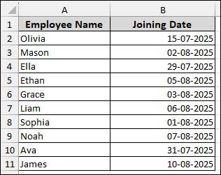
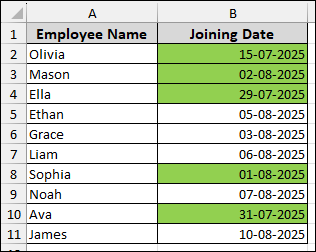
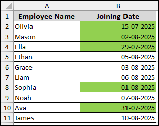
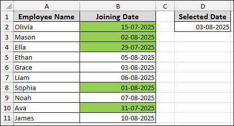
Suppose we have a list of Employee Names and their Joining Date. Our goal is to highlight any joining date that is older than a specific date (03-08-25).
DATE Function
The DATE function allows you to specify a fixed date using year, month, and day arguments. Here, we will apply the DATE function to specify the date inside the formula box of conditional formatting. To apply conditional formatting, first select the cells you wish to format.
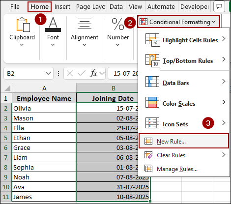
➤ Select the range B2:B11.
➤ Click Home > Conditional Formatting from the menu bar.
➤ From the dropdown menu, choose New Rule.
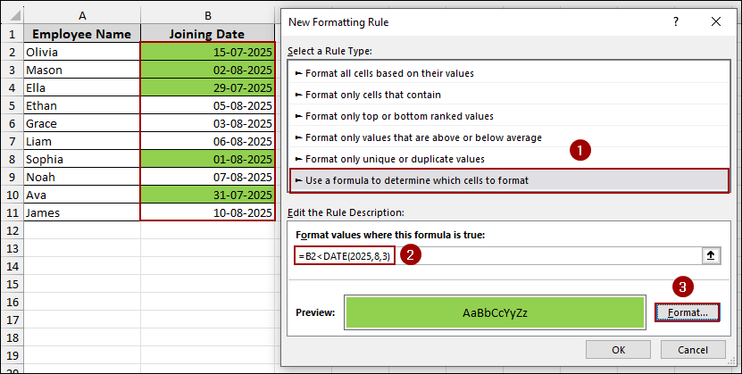
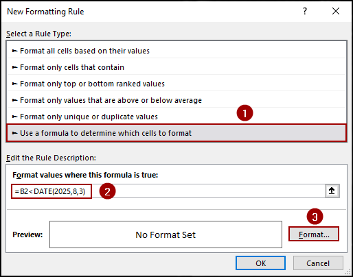
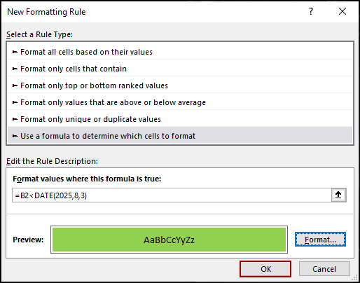
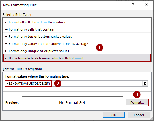
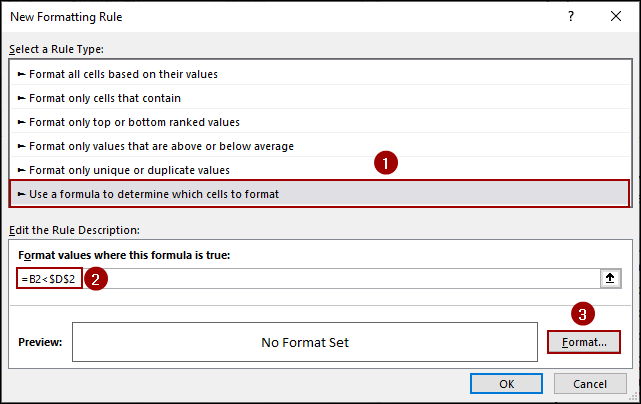
In the New Formatting Rule dialog box, we will define our rule using a formula.
➤ Select the option Use a formula to determine which cells to format.
➤ In the Format values where this formula is true field, enter the formula.
=B2<DATE(2025,8,3)
➤ Click the Format button.
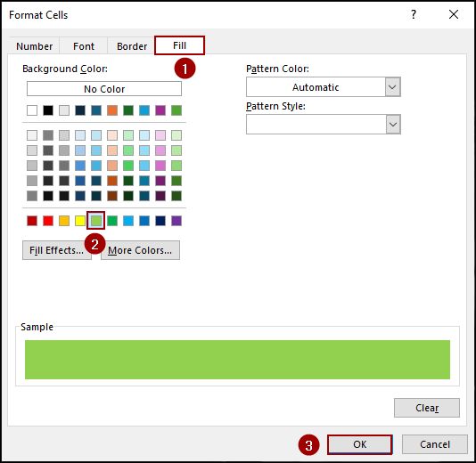
➤ In the Format Cells dialog box, go to the Fill tab and choose a color (e.g., light green).
➤ Click OK to confirm the format.
➤ Then hit OK again in the New Formatting Rule dialog box.
As a result, any joining date in the selected range that is older than August 3, 2025, will be highlighted with the chosen fill color.
TODAY Function
The TODAY function provides the current date in Excel. This is useful when you want your conditional formatting to update automatically each day.
To set up this rule, ensure your range B2:B11 is still selected.
➤ Following the previous method, go to Home > Conditional Formatting > New Rule.
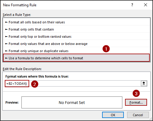
➤ In the New Formatting Rule box, select Use a formula to determine which cells to format.
➤ In the Format values where this formula is true field, write down the formula.
=B2<TODAY()
➤ Click the Format button.
➤ Choose your desired formatting (e.g., a different shade of green), and click OK twice.

Thus, dates older than the today’s date will be highlighted, and this highlighting will update daily.
DATEVALUE Function
The DATEVALUE function converts a date represented as text into an Excel serial number. This is useful if your certain date is initially provided as text.
Make sure your range B2:B11 is still selected.
➤ Following the previous method, go to Home > Conditional Formatting > New Rule.
➤ In the New Formatting Rule box, select Use a formula to determine which cells to format.
➤ In the Format values where this formula is true field, write down the formula.
=B2<DATEVALUE("03/08/25")
➤ Click the Format button.
➤ Select your desired formatting, and click OK twice.

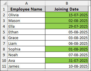
Finally, dates older than August 3, 2025, as text, will now be highlighted with the chosen format.
Using Cell Reference to Check Dates Older Than a Certain Date
Instead of writing a date into the formula, you can use a cell reference. This makes your conditional formatting flexible, allowing you to change the certain date simply by updating a single cell.
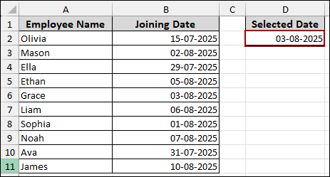
Suppose we have the same dataset and a selected date in cell D2, 03-08-2025 as our certain date.
➤ Select your range B2:B11, following the previous method, go to Home > Conditional Formatting > New Rule.
➤ In the New Formatting Rule box, select Use a formula to determine which cells to format.
➤ In the Format values where this formula is true field, write down the formula.
=B2<$D$2
➤ Hit the Format button.
➤ Select your desired formatting (e.g., light green fill), and press OK twice.

As a result, all joining dates in the range B2:B11 that are older than the date specified in cell D2 will be highlighted. To change which dates are highlighted, simply update the date in cell D2.
Frequently Asked Questions
What if the cell is blank? Will it be highlighted?
No, blank cells will not be highlighted by default with the < comparison. But to make sure, you can use this type of formula: =AND(A2<DATE(2025,7,20),A2<>””)
Can I highlight only weekends or holidays that are past a certain date?
You can highlight weekends with this formula: =AND(A2<TODAY(),WEEKDAY(A2,2)>5). For holidays, you don’t need a list of dates and you can use the MATCH function too.
Does Excel conditional formatting work with time values too (e.g., 2 PM)?
Yes, but time is treated as a decimal. To compare times apply this formula: =A2<TIME(14,0,0). This highlights times before 2:00 PM.
Concluding Words
Above, we have explored various methods for applying conditional formatting to highlight dates older than a certain date in Excel. By using functions like DATE, TODAY, DATEVALUE, or a simple cell reference, you can highlight data that quickly draw attention to important date related information. If you have any questions, feel free to leave them in the comments below.