Combining formulas in Excel allows you to find insightful summaries, which is useful for data analysis. This article covers five easy ways to combine two formulas in Excel with proper explanation and use cases.
To combine two formulas in Excel, follow the steps below:
➤ Enter the formula: =”Label1: “&TEXT(SUM(range), “format”)&”, Label2: “&TEXT(AVERAGE(range), “format”)
➤ Replace the “range” with the cells from which you want to find the sum and average values.
➤ Customize `format` to match your desired output (e.g., “$#,##0” for currency).
➤ Press the Enter button.
Here’s the summary of the five methods that we have used in this article. The first two methods show the way to combine text and numbers in a single cell. Then you’ll see the way of nesting functions. After that, we have talked about how to dynamically look up and add values with several conditions.
Combine Text and Number with Amersand Operator (&)
To combine text and numbers in a single cell, you can use the ampersand (&) operator between formulas. For example, in this dataset, we’ll display the total and average salary in a single cell. Follow the steps below.
Steps:
➤ Select the output cell (C15).
➤ Insert the following formula.
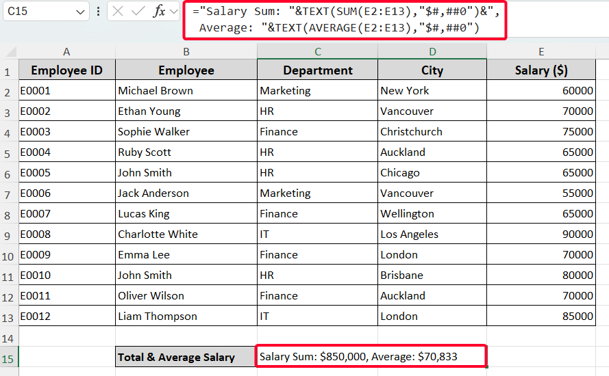
="Salary Sum: "&TEXT(SUM(E2:E13),"$#,##0")&", Average: "&TEXT(AVERAGE(E2:E13),"$#,##0")
➤ Press the Enter button.

The above output displays the sum and average of salaries in E2:E13 cells, formatted as currency.
Use CONCAT Function
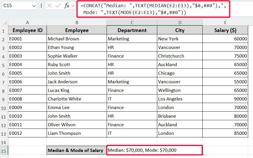
Instead of using the ampersand, you can also use the CONCAT function to combine text and formatted numbers. Here, we’ll show the median and mode of the salary. Just use the following formula.
=CONCAT("Median: ",TEXT(MEDIAN(E2:E13),"$#,##0"),", Mode: ",TEXT(MODE(E2:E13),"$#,##0"))
If you’re using Excel 2013 or an earlier version, use the CONCATENATE function. In that case, the formula will be as follows:
=CONCATENATE("Median: ", TEXT(MEDIAN(E2:E13), "$#,##0"), ", Mode: ", TEXT(MODE(E2:E13), "$#,##0"))
Nest IF Statements for Conditional Logic
When logical conditions are involved, you can nest multiple IF functions together.
Steps:
➤ Insert the following formula in the F2 cell.
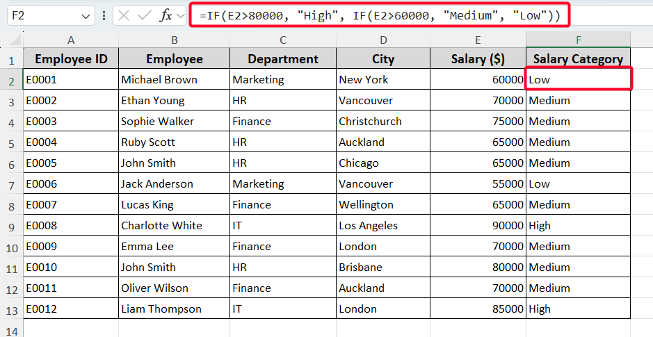
=IF(E2>80000, "High", IF(E2>60000, "Medium", "Low"))
This formula checks the salary in E2. If it’s above 80,000, it returns “High”. If it’s above 60,000, it returns “Medium”. Otherwise, it returns “Low”.
➤ After pressing the Enter button, use the Fill Handle tool to copy the formula to F13 cells.
Note:
You can nest up to 64 functions within a single formula, allowing for highly complex calculations. For example, combining IF, AND, and OR.
Use INDEX-MATCH Formula for Dynamic Lookup
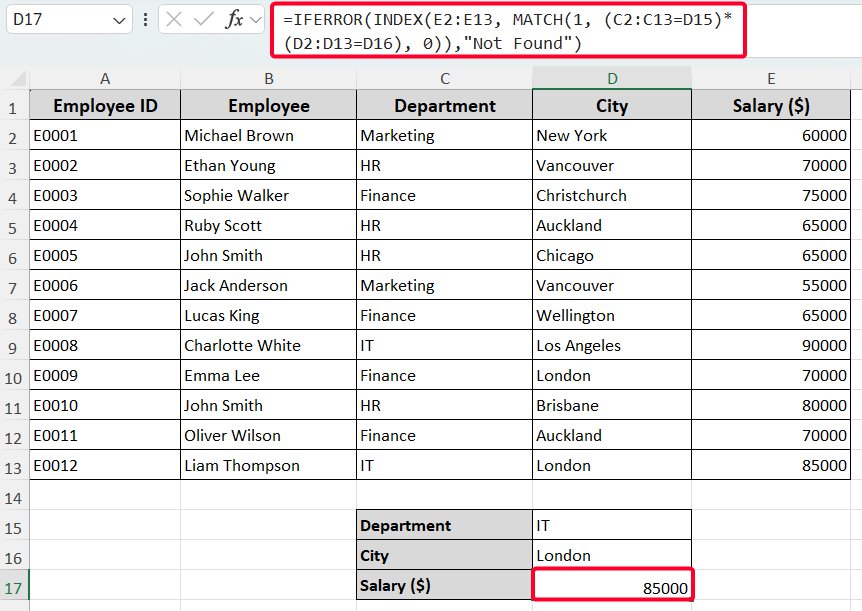
For dynamic lookup, for example, when you need to find a specific value based on multiple criteria, you can use the combination of the INDEX–MATCH formula. Like, we’ll find the salary of the “IT” department based on London city.
=IFERROR(INDEX(E2:E13, MATCH(1, (C2:C13=D15)*(D2:D13=D16), 0)),"Not Found")
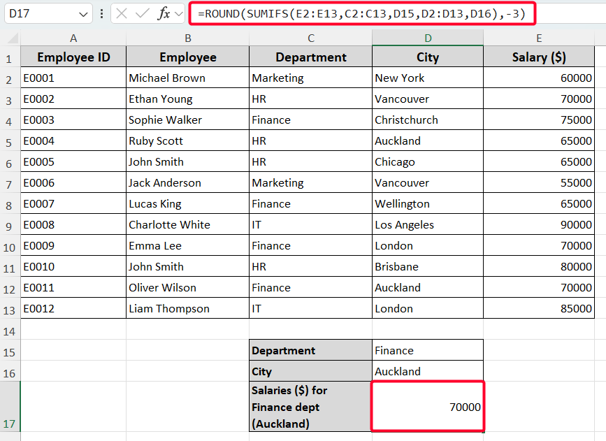
Combine Formulas to Sum Values with Multiple Conditions
You can use SUMIFS function to sum values based on multiple conditions. For example, we’ll sum the salaries of employees based in Auckland for the “Finance” department. Use the following formula.
=ROUND(SUMIFS(E2:E13,C2:C13,D15,D2:D13,D16),-3)
Frequently Asked Questions
Can I combine two formulas that each return TRUE/FALSE or logical results?
Yes. You can use logical operators like AND or OR. You can even use these logical operators with the IF function.
How do I combine date and time formulas?
To combine date and time formulas into a single cell, use the TEXT function. For example, the =TEXT(NOW(), “dd-mm-yyyy hh:mm:ss”) combines the NOW function with TEXT to format the result.
Is there a character limit for formulas in Excel?
Yes. Excel formulas have a character limit of 8,192 characters per cell in the formula bar.
Wrapping Up
This is how you can use the above-discussed methods to combine two formulas in Excel. Use those methods based on your requirement—from the ampersand to condition-based lookup. Hopefully, you have enjoyed the article. Feel free to download the practice workbook and share your thoughts in the comments!