Conditional formatting allows users to highlight the Excel cells based on the given conditions. This feature is quite beneficial for visual representation. For example, you can use it to highlight top scores, sales over a certain value, overdue tasks, higher values, etc. In all these cases, you can apply the conditional formatting feature to the selected cells.
To apply conditional formatting to the selected non-adjacent cells, follow the below steps. ➤ First select the B2 cell, then press the Ctrl button and select the D2 cell.
➤ Go to Home tab >> Conditional Formatting >> Highlight Cells Rules >> Greater Than…
➤ Put greater than value and press OK.
What Is Conditional Formatting in Excel?
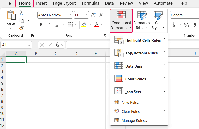
Conditional formatting is a feature in Excel that automatically changes the appearance of cells based on the conditions you set. You can find it in the Styles ribbon group under the Home tab. Alternatively, use the Alt + H + L buttons to open it quickly. The primary used options of this feature: Highlight Cells Rules, Top/Bottom Rules, Data Bars, Color Scales, and Icon Sets are visible. Besides, you will get the options to create, clear, and manage rules.
This article shows several ways to use conditional formatting: on cells not next to each other, on two separate columns, on a selected range of cells with formulas, and to find duplicates. Lastly, we’ll focus on the use of data bars option in the conditional formatting to the selected cells.
Apply Conditional Formatting to Selected Non-Adjacent Cells
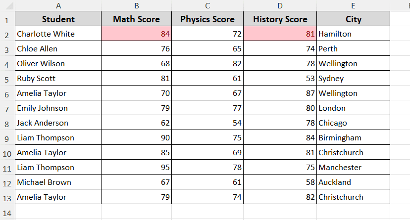
We have used the following dataset which shows student information along with their grades in three different subjects. We want to apply the conditional formatting to the selected non-adjacent cells.
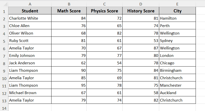
Now, we will highlight non-adjacent cells B2 and D2 only if their scores exceed 80.
Steps:
➤ First select the B2 cell, then press Ctrl button and select the D2 cell.
➤ Go to Home tab >> Conditional Formatting >> Highlight Cells Rules >> Greater Than…
➤ Put 80, as marked in the following image of the Greater Than pop-up window.
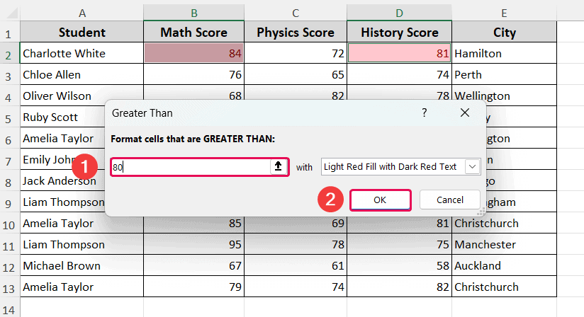
➤ Press OK.
Finally, you’ll get the following output where two cells are highlighted as the score is above 80.
Conditional Formatting Across Two Separate Columns
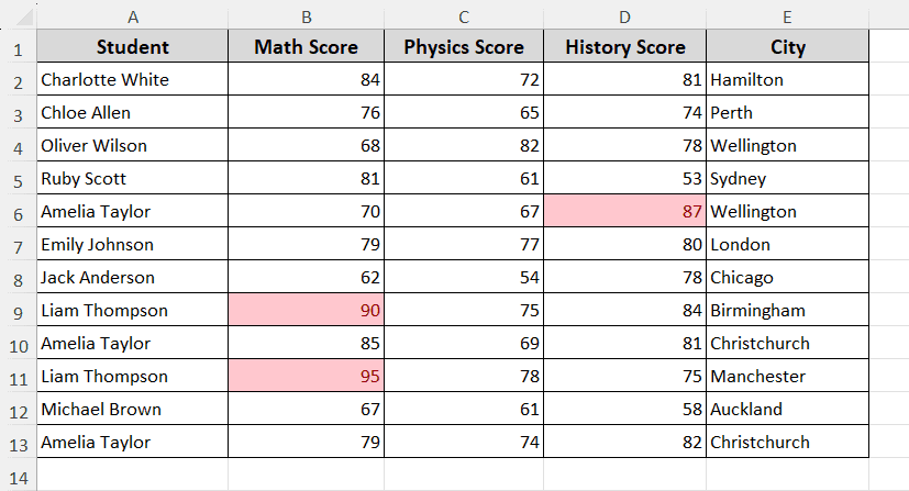
In this method, we will find the top 3 scores across two separate columns B & D.
Steps:
➤ At the beginning, select the B column (B2:B13 cells), then press Ctrl button and select the D column (D2:D13 cells).
➤ Go to Home tab >> Conditional Formatting >> Top/Bottom Rules >> Top 10%…
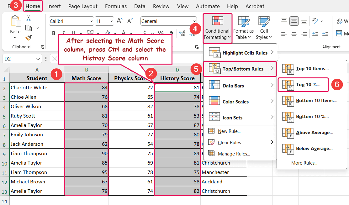
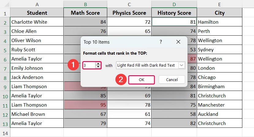
➤ Enter the value as 3, as shown in the following image of the Top 10 Items dialog box.
➤ Press OK.
So that the output will be as follows.
Use Conditional Formatting for Selected Range of Cells with Formulas
This method is slightly different. In this method, we will highlight the entire row that meets the criteria: the student’s name must be “Liam Thompson”, and the city must be “Birmingham”.
Steps:
➤ First select the A2:E13 cell range.
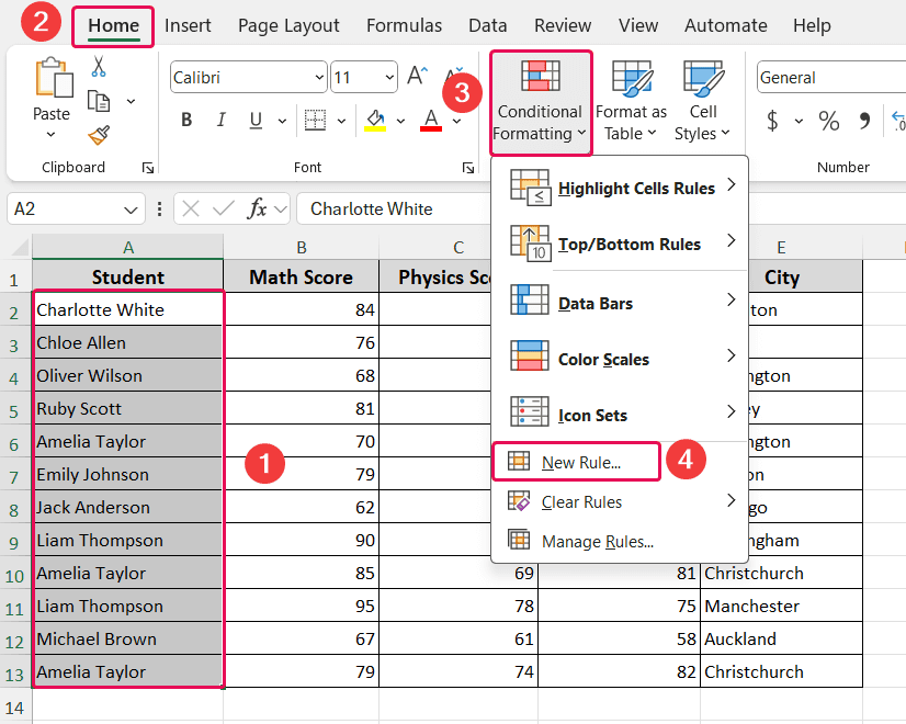
➤ Go to Home tab >> Conditional Formatting >> New Rule…
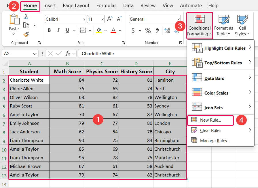
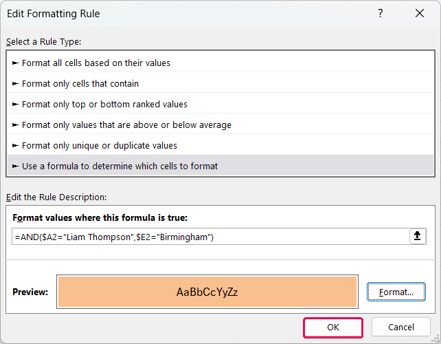
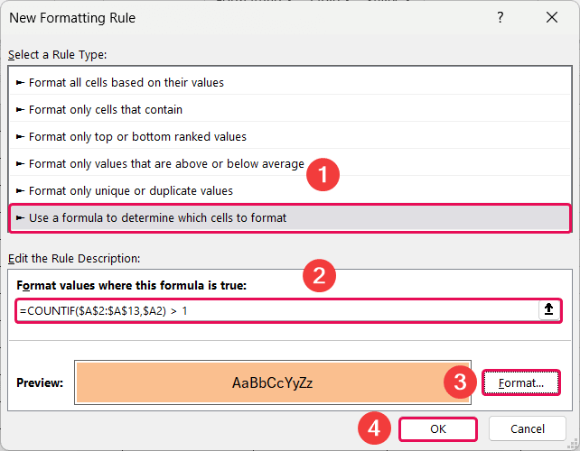
➤ Pick the Use a formula to determine which cells to format option and enter the following formula in the formula box.
=AND($A2="Liam Thompson",$E2="Birmingham")
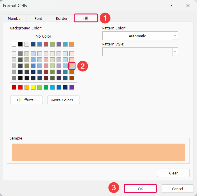
➤ Click on the Format… option.

➤ Go to the Fill tab, pick a suitable color, and press OK.
➤ Just press OK.
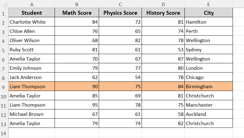
You will then see that row 9 is highlighted.
Find Out Duplicates Using Conditional Formatting
This method finds duplicate entries in the “Student” column. For this, we’ll use the COUNTIF function.
Steps:
➤ Select A2:A13 cells.
➤ Go to Home tab >> Conditional Formatting >> New Rule…
➤ Then enter the following formula, set the format and press OK.
=COUNTIF($E$2:$E$13,$E2) > 1
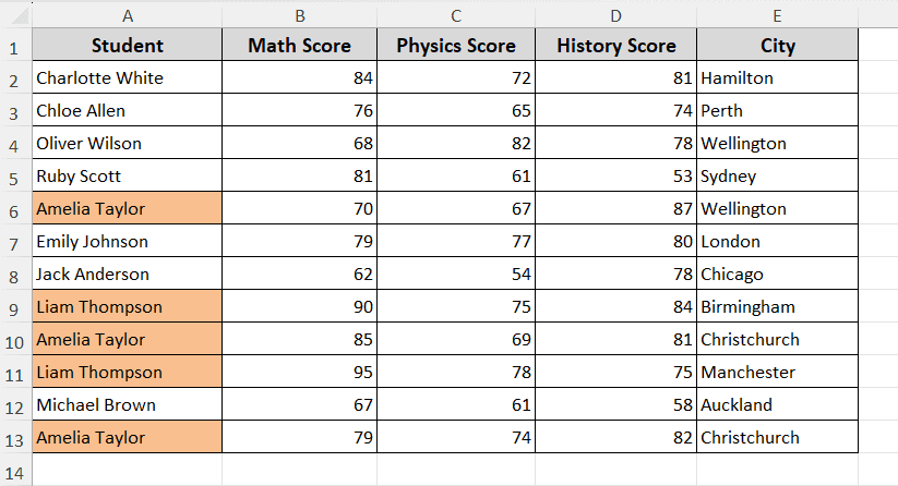
And you’ll get the following output.
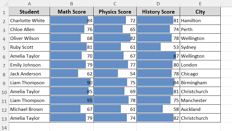
Add Data Bars to the Selected Cells for Conditional Formatting
If you want to get a visual representation of cell values, you can use the Data Bars option from the Conditional Formatting feature in Excel. This offers a comparison of the values, where longer data bars indicate higher values.
Steps:
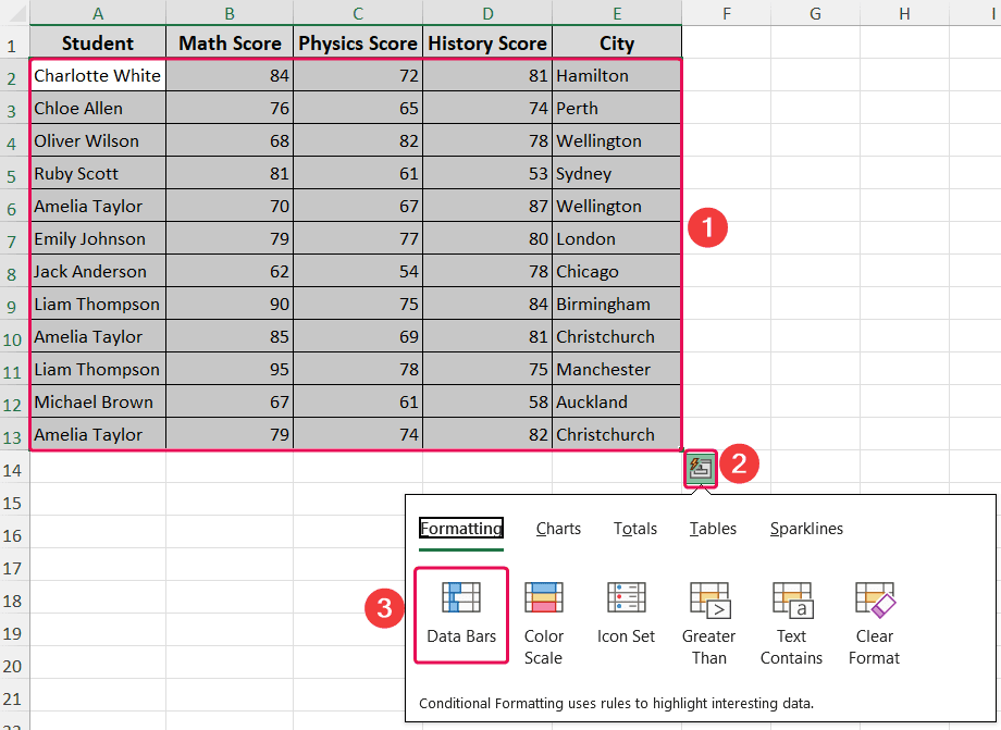
➤ Select the A2:E13 cells first.
➤ Soon, you’ll see a Quick Analysis Tool at the bottom-right corner of your selection. Also, you can use the Ctrl + Q buttons as the keyboard shortcut.
➤ Pick Data Bars icon.
After that you’ll get the following output.
FAQ
How to apply conditional formatting to a cell based on another cell?
Let’s say you want to highlight the A2 cell based on the cell value of B2. That means if the cell value of B2 is greater than 80, the A2 cell will be highlighted. To do this, go to Home >> Conditional Formatting >> New Rule… >> enter the formula:
=B2>80
How to apply conditional formatting to the selected cells so cells with a value greater than 400 are formatted using a light red fill?
To highlight cells with values greater than 400 using conditional formatting with a Light Red Fill, Go to Home tab >> Conditional Formatting >> Highlight Cells Rules >> Greater Than…In the “Greater Than” pop-up window, enter “400” as the value and select “Light Red Fill” from the options on the right.
Can we copy conditional formatting from one cell to another?
Yes, you can copy conditional formatting from one cell to another in Excel. Here is the way:
➤ Select the cell where you have already applied the conditional formatting.
➤ Click the Format Painter button in the Home tab (from the Clipboard group).
➤ Choose the cell where you want to copy the conditional formatting.
Wrapping Up
In this article, we explored five ways to use conditional formatting: on cells not next to each other, on two separate columns, on a selected range of cells with formulas, and to find duplicates. Additionally, we discussed the use of data bars option from the Quick Analysis tool. Feel free to download the practice file and share your thoughts and suggestions. This article shows.