

Converting an entire column to number is often necessary in Excel to ensure consistency and accurate calculation across the dataset. By using Excel’s built-in tools and functions, we can perform this operation with ease.
Follow the steps below to convert the entire column to numbers in your Excel Dataset.
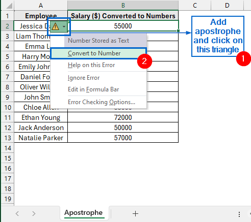
➤ In your dataset, head to the column you want to convert to numbers and place an apostrophe (‘) before each value.
➤ Next, select the entire column and click on the error indicator located at the top left corner of the cells.
➤ From the dropdown menu, select the Convert to Number option.
In this article, we will learn eight effective methods of converting an entire column to number in Excel.
Use Apostrophes to Convert Column to Number
In the sample dataset, we have a worksheet called “Employee Salary” containing information about Employee names and their corresponding Salary. By using an apostrophe (‘) together with the Convert to Number option, we will transform the salary values in column B into numbers. The modified dataset will be stored in a separate “Apostrophe” worksheet.

Convert to Number is an Excel feature that allows users to quickly change stored values into actual numeric data which can be used in calculations.
Steps:
➤ Head to the Apostrophe worksheet, select cell B2 and add an apostrophe (‘) before the value.
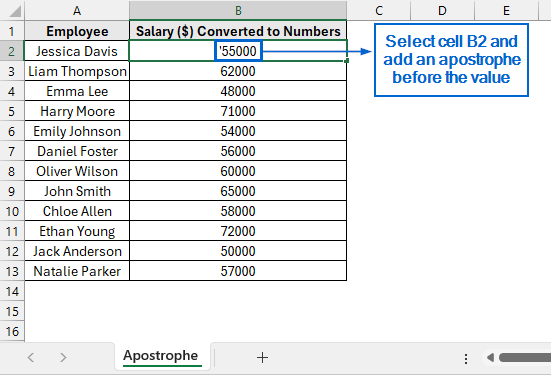
➤ Repeat the same step for cells B3 to B13.
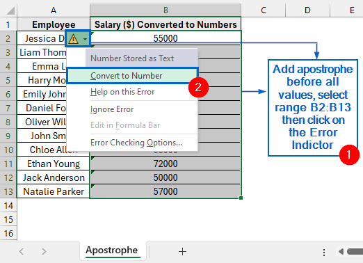
➤ Next, select the range B2:B13 and click on the Error Indicator situated at the top left corner of the cell.
➤ Then, select the Convert to Number option from the dropdown menu.
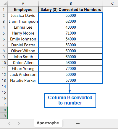
➤ All values in column B should now be converted to numbers.
Convert Column to Number By Multiplying 1
By multiplying a value by 1, Excel forces it to be recognized as a number, ensuring it can be used properly in calculations. Working with the same dataset, we will now multiply all cells in range B2:13 by 1 and convert the entire column to number. We will display the modified dataset in a separate worksheet called “Multiply”.
Steps:
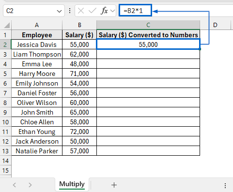
➤ Head to the Multiply worksheet, select cell C2, and put the following formula:
=B2*1
Note:
This simple formula multiplies the value in cell B2 by 1, converting it into a numeric value.
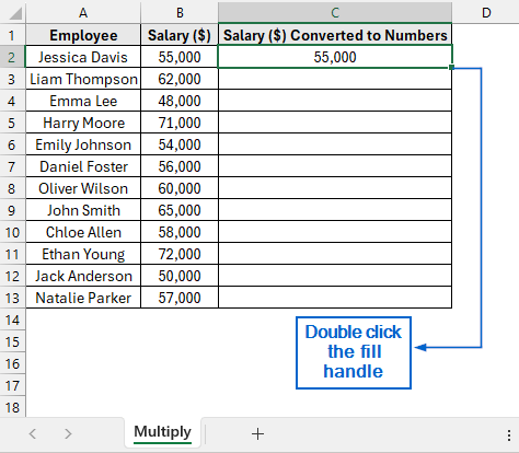
➤ Select cell C2 again and double-click the fill handle to apply the formula across the entire column.
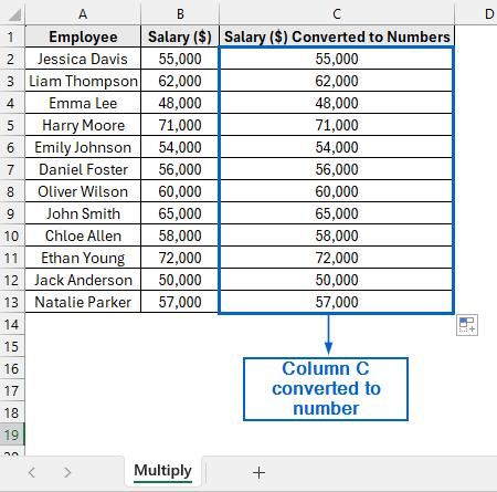
➤ Column C should now display the salary converted to number.
Add Zero to Convert Column to Number
Just like the previous method, adding zero to a value also forces Excel to treat it as a number. Using the same dataset again, we will convert the values in column B to number by adding zero to the values. The modified dataset will be stored in a separate “Add” worksheet.
Steps:
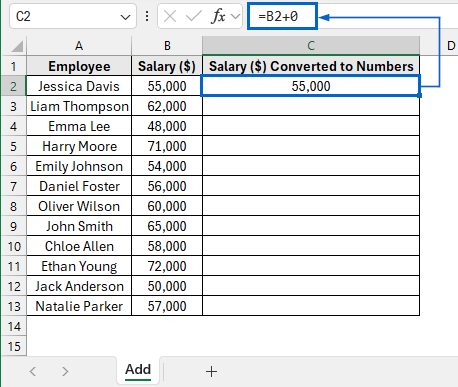
➤ Go to the Add worksheet, select cell C2, and paste the following formula:
=B2+0
Note:
This simple formula adds 0 to the value in cell B2, converting it into a numeric value.
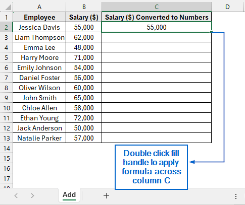
➤ Select cell C2 again and double-click the fill handle to copy the formula down the entire column.
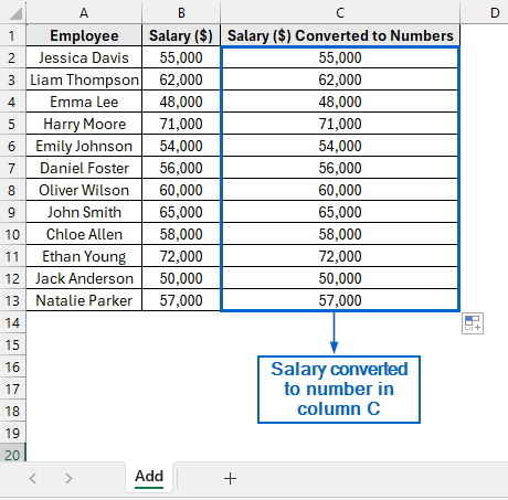
➤ Column C should now display the salary converted to number.
Divide Value by 1 to Convert Column to Number
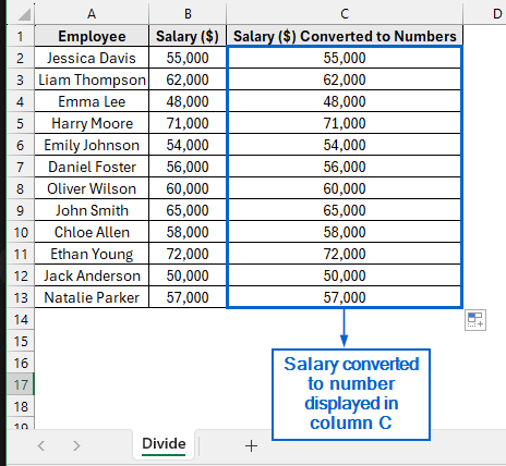
Like the previous methods, dividing a value by 1 also converts it into numeric form. Using the same dataset again, we will now divide all values in column B by 1 to convert them into numbers. The updated dataset will be stored in a separate “Divide” worksheet.
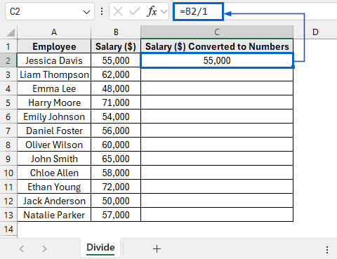
➤ Head to the Divide worksheet, select cell C2, and enter the following formula:
=B2/1
Note:
This formula divides the value in cell B2 by 1 and converts it into a numeric value.
➤ Select cell C2 again and double-click the fill handle to apply the formula across column C.
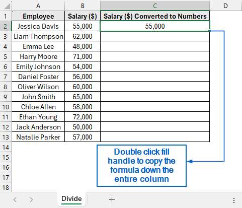
➤ All values in column C should now be converted to numbers.
Apply Number Formatting to Transform Column into Number
Excel’s Number Formatting allows users to customize how numbers are displayed, enabling them to add decimal places, currency symbols, or percentages without changing the original value.
Using the same dataset, we will now apply number formatting to column B and transform the entire column into number. We will show the updated dataset in a separate “Number Format” worksheet.
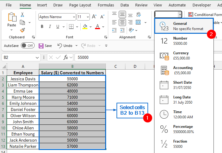
➤ Head to the Number Format worksheet and select cells B2 to B13.
➤ From the main menu, navigate to Number group and choose General from the dropdown menu.
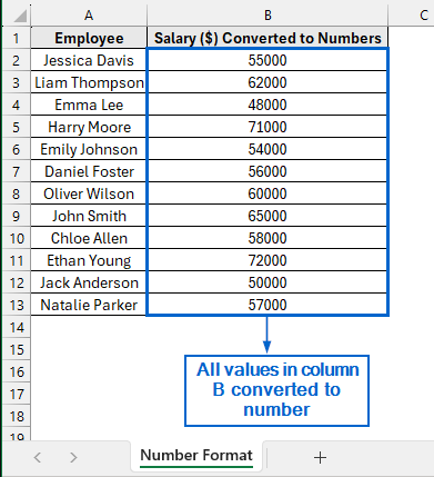
➤ All values in column B are now converted to number.
Use the Paste Special Tool to Transform Column into Number
Paste Special is a useful Excel tool that lets users choose how copied data is pasted. We will work with the same dataset and convert the values in column B to numbers using the Paste Special tool. The modified dataset will be displayed in a separate “Paste Special” worksheet.
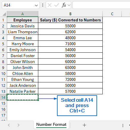
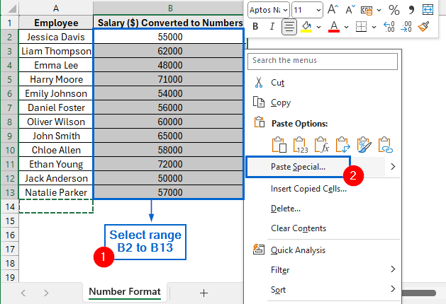
➤ Go to the Paste Special worksheet, select cell A14 and press Ctrl + C to copy it.
➤ Next, select the range B2 to B13, right-click to open the context menu and click on Paste Special.
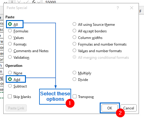
➤ In the Paste Special dialogue box, select All under Paste, choose Add under Operation, and click OK to apply the changes.
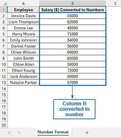
➤ Column B will now display the values converted into numbers.
Convert Column to Number Using Text to Column Feature
The Text to Column feature in Excel allows users to split the contents of a cell into multiple columns based on a specified delimiter, such as spaces, commas, or tabs.
Using the same dataset again, we will use the Text to Column feature to transform the value in column B into number.
Steps:
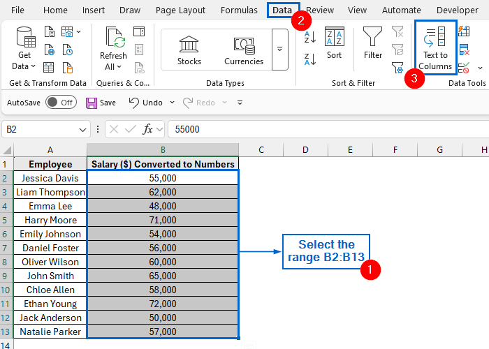
➤ Go to the Text to Column worksheet, select range B2:B13, and from the main menu navigate to Data >> Text to Columns.
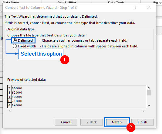
➤ Click on Delimited from the Convert Text to Columns Wizard dialogue box and press Next.
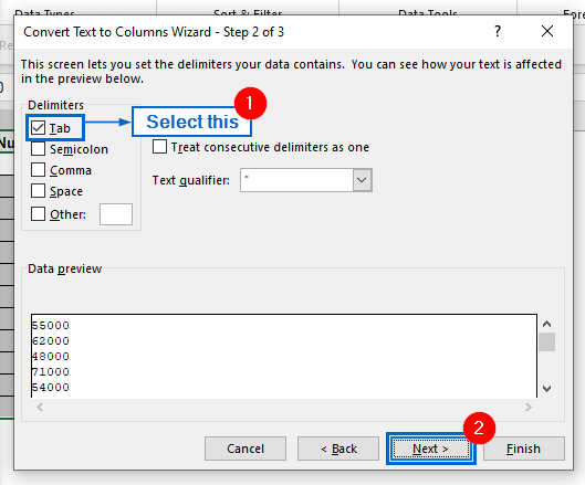
➤ Select Tab as the delimiter and click Next again.
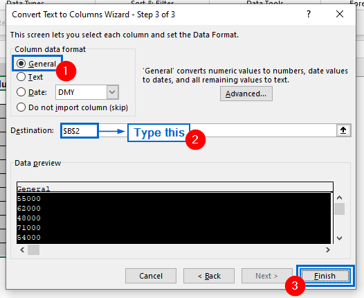
➤ Finally, set the Column data format to General, type $B$2 in the destination box, and click Finish to complete the process.
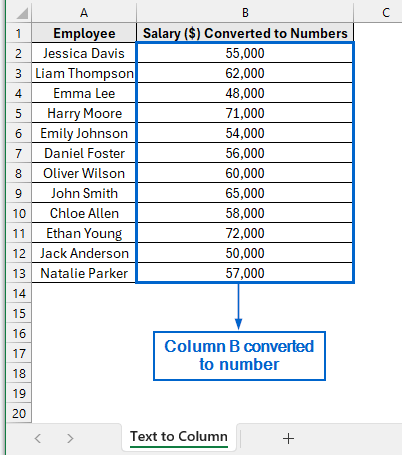
➤ All values in column B are now converted to numbers.
Use the VALUE and TRIM Functions to Convert Entire Column to Number
The VALUE function in Excel converts text that appears as a number into an actual numeric value, while the TRIM function removes extra spaces from text.
Working with the same dataset again, we will now use VALUE with TRIM functions to convert the values in column B into numbers and display the results in column C. We will store the modified dataset in a separate worksheet called “VALUE With TRIM”.
Steps:
➤ Go to the VALUE With TRIM worksheet, select cell B2, and paste the following formula:
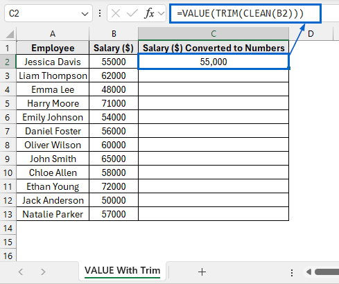
=VALUE(TRIM(CLEAN(B2)))
➧ CLEAN(B2) removes all non-printable or hidden characters from the value in cell B2.
➧ TRIM(...) then removes any extra spaces, leaving only single spaces between digits.
➧ VALUE(...) finally converts the cleaned text into a proper numeric value.
➤ Next, select cell C2 again and double-click the fill handle to apply the formula to the entire column.
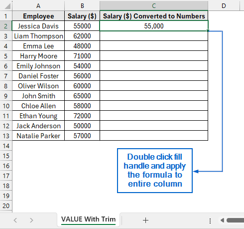
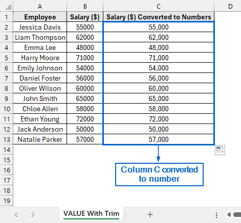
➤ Value converted to numbers is now displayed in column C.
Downloadable Resources
Get our practice workbook or necessary files that we have worked with to prepare this article.
Convert Entire Column to Number.xlsx
Frequently Asked Questions
Which is the Quickest Method For Dealing With Large Datasets?
For large datasets, the Paste Special and Text to Columns methods are the quickest options. Both can handle an entire column in a single step without relying on formulas, making them highly efficient.
Do These Methods Work With Blank Cells in the Column?
Yes. Blank cells remain unaffected in all of the above methods. Excel automatically skips empty cells during the conversion process, ensuring that only valid entries are converted into numeric values.
Concluding Words
Knowing how to convert an entire column to number is crucial for tasks like applying formulas, creating charts, or performing data analysis.
In this article, we have discussed eight effective methods of converting an entire column to number in Excel, including using Apostrophe, Multiplication, Addition, Division, Number Formatting, Paste Special tool, Text to Column feature and combining VALUE with TRIM functions. Feel free to try all methods and select one that best aligns with your needs.