In Excel, a custom number format allows you to control how numbers, text, and dates appear in your worksheet without changing their actual values. For example, you might want positive numbers to appear in green, negative numbers in red, and zeros in gray. Instead of applying conditional formatting rules, you can achieve this using Excel’s Custom Number Format feature.
In this article, you’ll learn how to apply a custom number format with multiple conditions in Excel. We’ll cover common scenarios like formatting positive, negative, and zero values differently, and adding text labels within numbers.
Here’s how custom number format with multiple conditions works in Excel:
➤ Open your dataset in Excel.
➤ Select the range B2:B11.
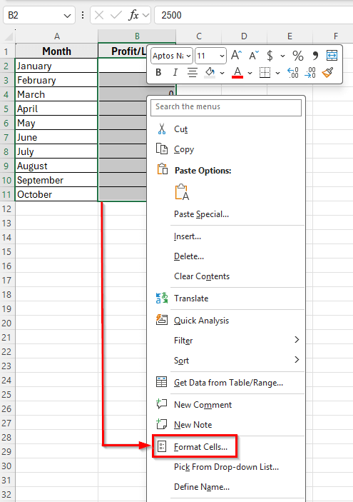
➤ Press Ctrl + 1 on your keyboard or right-click and choose Format Cells.
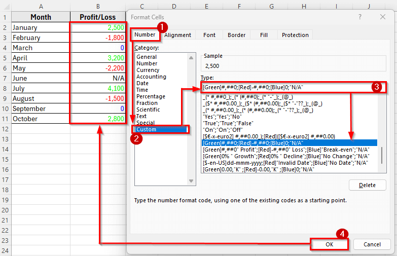
➤ In the Format Cells dialog box, go to the Number tab and select Custom.
➤ In the Type box, enter this custom format:
[Green]#,##0;[Red]-#,##0;[Blue]0;”N/A”
➤ Click OK. Now, Excel will instantly format the values like Positive numbers turn into Green, negative numbers display as Red with minus sign, zero values turn into Blue, and text values display as N/A.
Apply Custom Number Format with Multiple Conditions
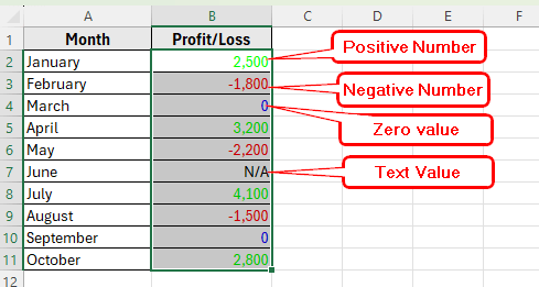
In the following dataset, we have a simple business record that tracks monthly profit and loss values. Column A lists the Months, and Column B shows the Profit/Loss amounts.
Some months have positive profits, others have losses, a few show zero, and one entry is marked as N/A (not available). This variety makes it perfect for demonstrating how to apply custom number formats with multiple conditions in Excel.
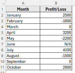
We’ll use this dataset to format positive numbers in green, negative numbers in red, zero values in gray, and text entries as N/A.
The easiest way to format numbers differently based on conditions is by using Excel’s Custom Number Format feature. With this method, you can apply different colors and display styles for positive values, negative values, zeros, and even text.
Here’s how to apply this method:
➤ Open your dataset in Excel.
➤ Select the range B2:B11.
➤ Press Ctrl + 1 on your keyboard or right-click and choose Format Cells.
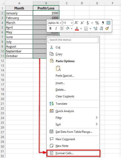
➤ In the Format Cells dialog box, go to the Number tab and select Custom.
➤ In the Type box, enter this custom format:
[Green]#,##0;[Red]-#,##0;[Blue]0;”N/A”
➤ Click OK.
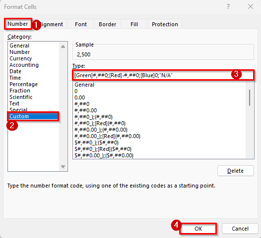
➤ Now, Excel will instantly format the values like positive numbers turn into Green, negative numbers display as Red with minus sign, zero values turn into Blue, and text values display as N/A.
Add Text Labels with Custom Number Format
Sometimes it’s not enough to just show numbers in different colors. You may also want to add descriptive labels like Profit, Loss, or Break-even directly in the same cell. This can make your dataset more informative without adding extra columns.
Here’s how to apply this method:
➤ Open your dataset in Excel.
➤ Select the range B2:B11.
➤ Press Ctrl + 1 or right-click and select Format Cells.
➤ In the Format Cells dialog box, go to the Number tab and choose Custom.
➤ In the Type field, enter this custom format:
[Green]#,##0″ Profit”;[Red]-#,##0″ Loss”;[Blue]”Break-even”;”N/A”
➤ Click OK.
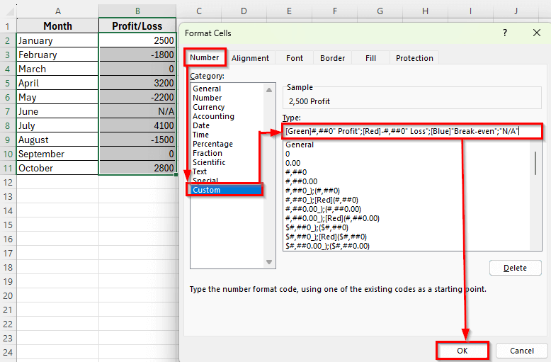
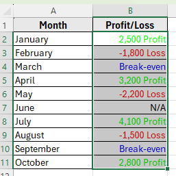
➤ Now, Excel will display your dataset as follows such as Profit display as Green, Loss display as Red, 0 display as text Break-even in Blue, and N/A text stays as it is.
Format Percentages with Multiple Conditions
If your dataset contains percentages, you can apply custom number formats to highlight whether a value shows growth, decline, or no change. This is especially useful for financial reports, sales growth, or performance tracking.
Instead of showing plain percentages, you can add text labels such as Growth, Decline, or No Change to make the results more meaningful.
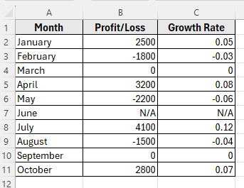
First, let’s extend our dataset by adding a new Column C labeled as Growth Rate %. Suppose this column contains monthly growth percentages.
Here’s how to apply it:
➤ Open your dataset in Excel.
➤ Select the range C2:C11.
➤ Press Ctrl + 1 or right-click and Format Cells.
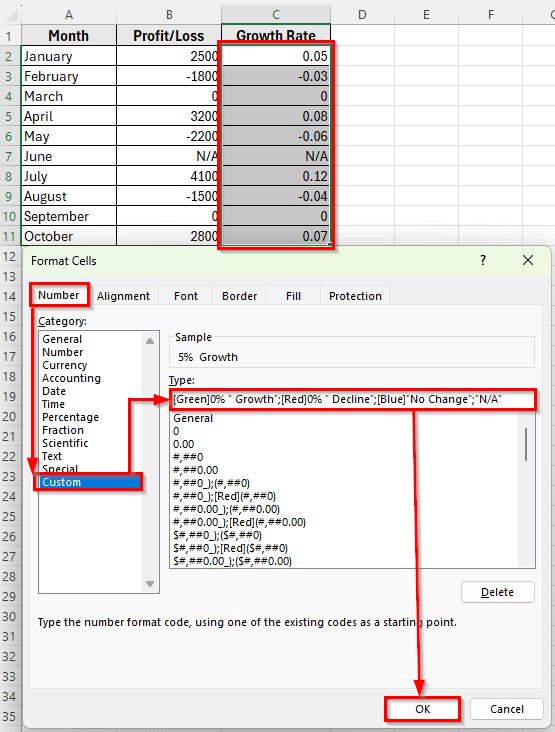
➤ In the Format Cells dialog box, go to the Number tab and choose Custom.
➤ In the Type field, enter this custom format:
[Green]0% ” Growth”;[Red]0% ” Decline”;[Blue]”No Change”;”N/A”
➤ Click OK.
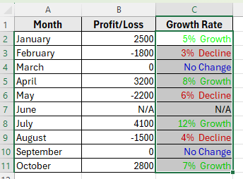
➤ Now, Excel will display your growth rates like Growth display as Green, Decline as Red, No Change as Blue, and N/A text remain unchanged.
Apply Custom Number Format to Dates
Excel stores dates as numbers in the background. By default, dates appear in a standard format (like 1/15/2025), but with custom number formats, you can control exactly how they display.
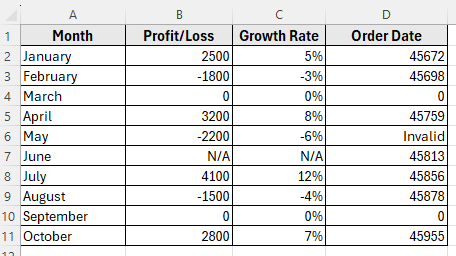
For example, you might want the regular dates to show in the full date format like 15-Jan-2025. Blank or zero values to display as No Date. Text entries to remain unchanged.
Add a new Column D as Order Date to our dataset with some valid dates, zeros, and text.
Here’s how apply this method:
➤ Open your dataset in Excel.
➤ Select the range D2:D11.
➤ Press Ctrl + 1 .
➤ In the Format Cells dialog box, go to the Number >> Custom.
➤ In the Type field, enter this custom format:
[$-409]dd-mmm-yyyy;[Red]”Invalid Date”;[Blue]”No Date”;”N/A”
➤ Click OK.
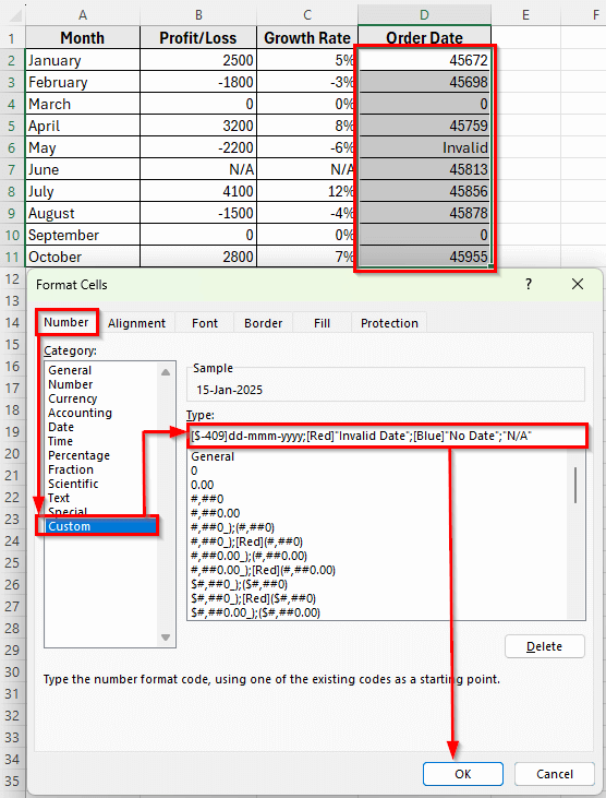
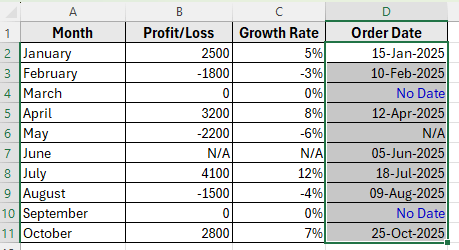
➤ Now, Excel will format your dates like 1/15/2025 to 15-Jan-2025 as a normal date. No Date displays as blue, and N/A text remains unchanged.
Frequently Asked Questions
How to custom number format in Excel?
To apply a custom number format in Excel:
➤ Select the cells you want to format.
➤ Press Ctrl + 1 or right-click and choose Format Cells.
➤ Go to the Number tab and select Custom.
➤ In the Type box, enter your custom number format code:
[Green]#,##0;[Red]-#,##0;[Blue]0;”N/A”
➤ Click OK to apply the format. This will automatically format positive numbers, negative numbers, zeros, and text according to your rules.
What is a custom number format in Excel?
A custom number format is a way to control how numbers, text, or dates are displayed in Excel cells without changing the actual values. You can apply colors, symbols, text labels, and even scale numbers automatically based on conditions.
How many conditions can I use in a custom number format?
Excel supports four sections in a custom number format such as Positive, Negative, Zero, and Text. Each section defines how Excel displays values in that category. For more complex rules, use Conditional Formatting.
Wrapping Up
Using custom number formats in Excel makes your data more readable and easier to interpret. You can apply colors, add text labels, format percentages, and display dates clearly. These formats do not change the actual values, so your calculations remain accurate.
With these techniques, you can make your reports look cleaner and more professional. Once you get comfortable with custom number formats, apply them in your dataset. It is a simple way to organize and highlight important information.