Sometimes we need to delete filtered rows. It is a useful thing when you want to remove specific data and don’t want to affect the rest of your worksheet. This is common when cleaning large datasets if necessary and where only certain rows meet a specific condition. The conditions can vary such as deleting all rows with “Zero Sales” or “Inactive” status.
To delete filtered rows in excel, follow these steps:
➤ Apply a filter to your dataset using Data > Filter.
➤ Filter for the values you want to delete (e.g., “Inactive” or “Zero”).
➤ Select the filtered rows, right-click, and choose Delete Row.
In this article, we’ll see four methods to delete filtered rows in Excel. We will use manual deletion, Go To Special etc.
Using Excel Basic Filter and Delete
This is one of the simplest and most effective ways we think to delete filtered rows in Excel. It’s very effective when you want to permanently remove some rows that meet a specific condition (e.g., “Absent” attendance) from a dataset.
Steps:
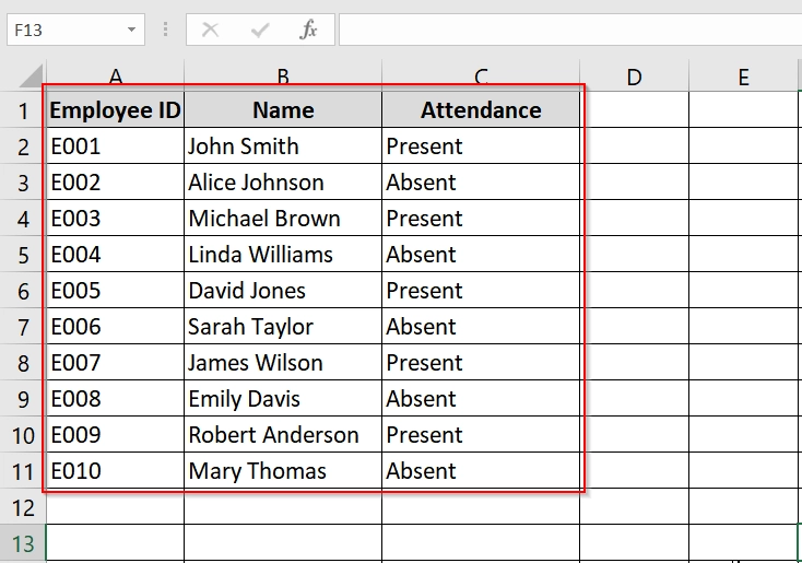
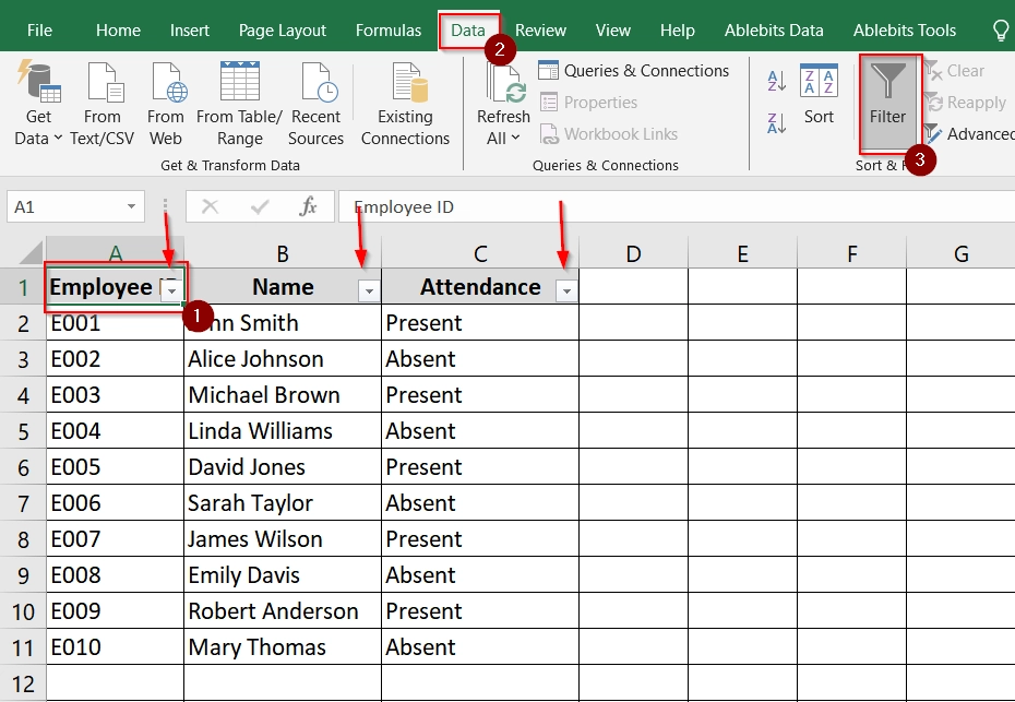
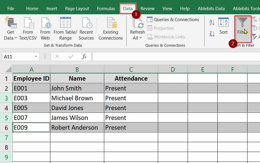
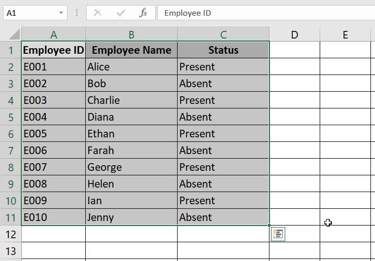
➤ Open your excel sheet. We will use the Employee Attendance table from Cell A1:C11.
➤ Select any cell in your dataset (e.g., A1).
➤ Go to the “Data” tab in the ribbon.
➤ Click on the “Filter” button. Small dropdown arrows will appear in the header row.
➤ Click on the dropdown in the “Attendance” column (C1). Uncheck everything except “Absent”. Click OK.
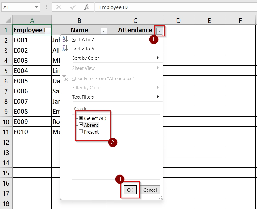
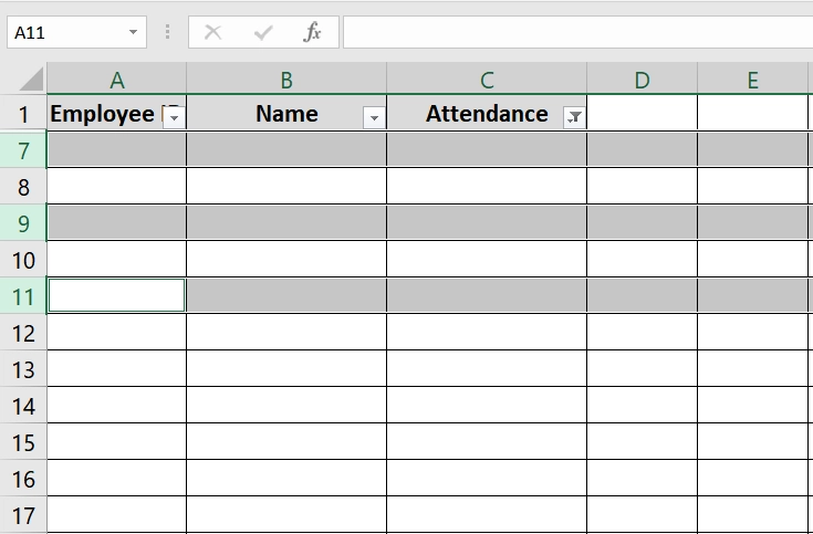
➤ Only the rows with “Absent” will be visible.
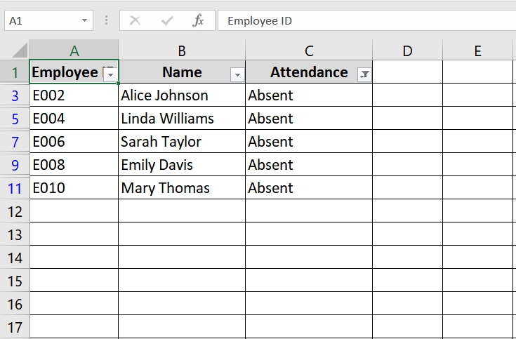
➤ Click on the row numbers on the left to highlight all visible filtered rows. You can click and drag from the first to last visible row.
For example, select rows 3, 5, 7, 9, 11 (those are Absent).
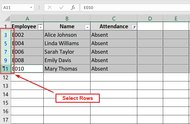
➤ Right-click on the highlighted rows. Select “Delete Row” (or press Ctrl + –).
➤ Go back to the “Data” tab and click the “Filter” button again to remove the filter and view all remaining data.
Note:
This method deletes rows permanently and you won’t be able to recover them without Undo.
Applying Special & Visible Cells Only Options To Delete Filtered Row
Apply Special & Visible Cells Only options to select and delete only the visible (filtered) cells in Excel. It’s helpful when some rows are hidden through filters, and you want to remove the visible (matching) data safely without touching hidden rows. It works well for datasets like sales, inventory, attendance sheets etc.
Steps:
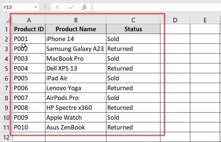
➤ Open your excel sheet and make sure your dataset is ready and contains headers in the first row. In this example, data is from cells A1:C11.
➤ Click on any cell in your dataset (e.g., A1).
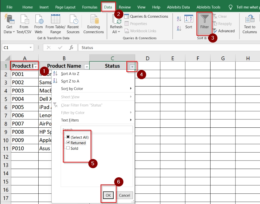
➤ Go to the “Data” tab.
➤ Click on the “Filter” icon.
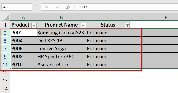
➤ In the “Status” column (C1), filter to show only “Returned” rows.
➤ Click and drag to select the visible rows in the filtered view (A2:C11 depending on which rows appear). Make sure not to include the header row unless you want to delete it too.
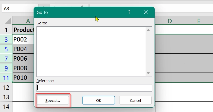
➤ With the filtered rows selected, press F5 on your keyboard (or Ctrl + G). Click on the “Special” button.
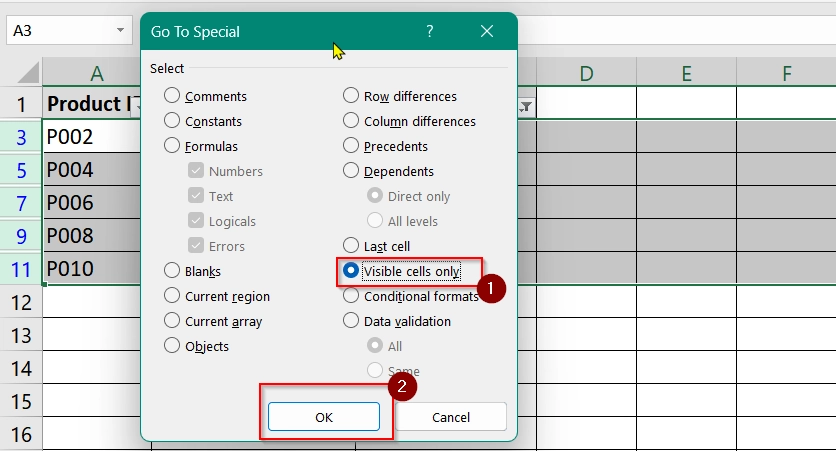
➤ In the pop-up, choose “Visible cells only” and click OK.
➤ Now that only visible cells are selected, right-click on any of the row numbers. Choose “Delete Row” (or press Ctrl + –).
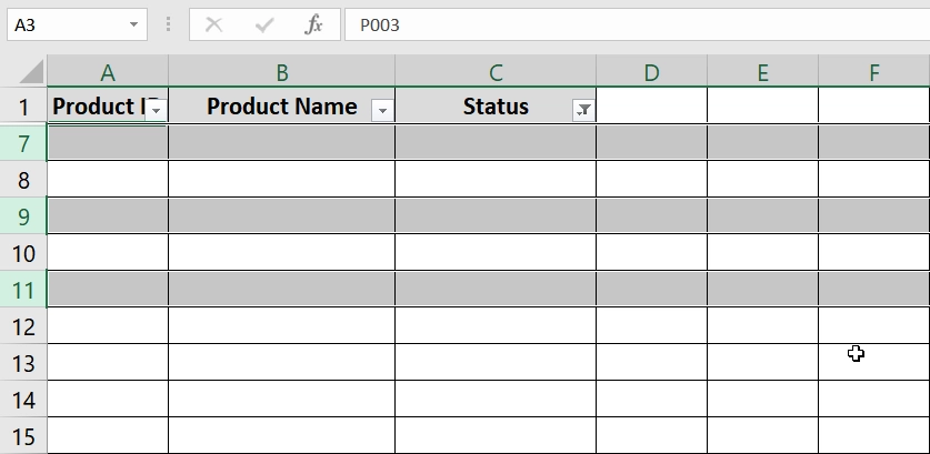
➤ Now, Return to the Data tab. Click on “Filter” again to remove all filtering. The dataset will now only show the non-deleted (unfiltered) rows.
Notes:
➧ “Go To Special” ensures that only visible (filtered) cells are selected. It protects any hidden data.
➧ If you skip this step and delete without using Go To Special, hidden rows will get deleted.
Delete Filtered Rows Using Power Query in Excel
Power Query is a powerful tool in Excel. It is widely used for data transformation and cleanup. When you want to permanently delete rows based on filters (like removing “Absent” records or rejected applications), Power Query is perfect. It loads data into an editor where you can filter and remove rows, then reload the clean version back into Excel.
Steps:
➤ Open your excel worksheet and make sure your data has headers (e.g., Employee ID, Name, Status). Select any cell in your table range (e.g., A1:C11).
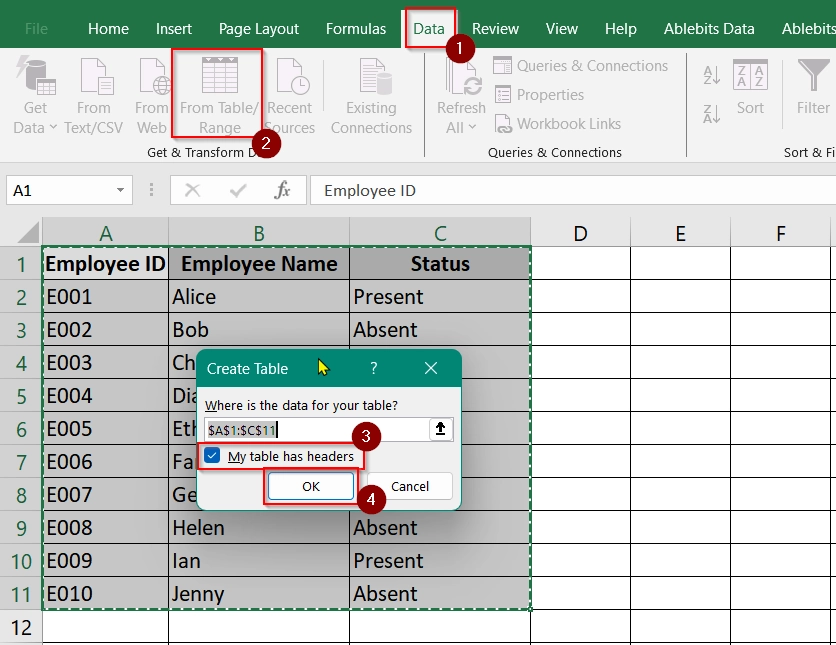
➤ Go to the Data tab on the ribbon.
➤ Click on “From Table/Range”.
➤ Check “My table has headers”.
➤ Click OK.
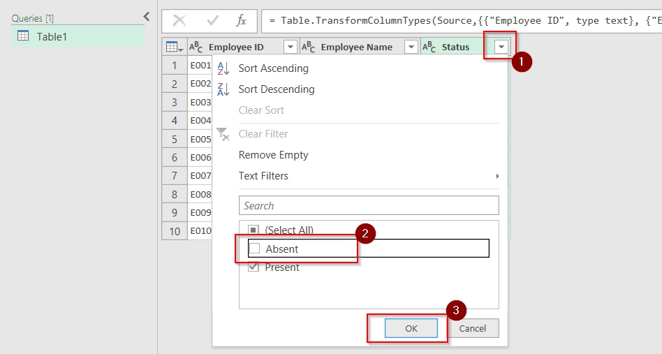
➤ In the Power Query editor, click the drop-down arrow in the Status column. Uncheck “Absent” to keep only “Present”. Click OK.
➤ Once the filter is applied, go to the Home tab. Click “Close & Load”.
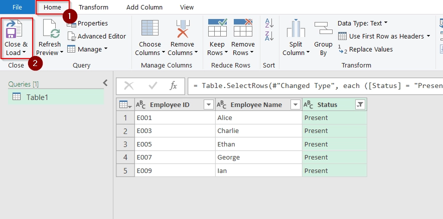
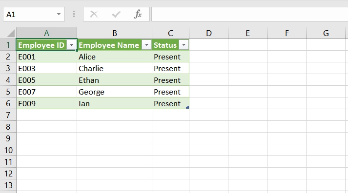
➤ The cleaned dataset will now be loaded into a new sheet in Excel.
Notes:
➧ Power Query does not delete rows in the original dataset directly. It creates a new version of the table after transformation.
➧ If your dataset changes frequently, you can refresh the Power Query output with updated filters using the “Refresh” option..
Filter Rows Using Advanced Filter and Delete
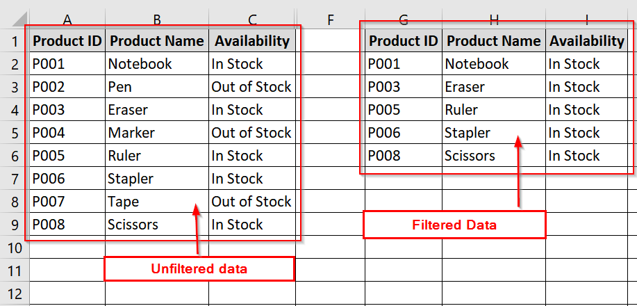
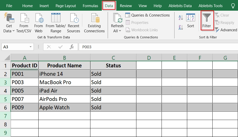
In this method we will use Excel’s Advanced Filter tool to extract and copy only the rows that match specific criteria (e.g., “In Stock”) to a new location. Then you delete the original table.
Steps:
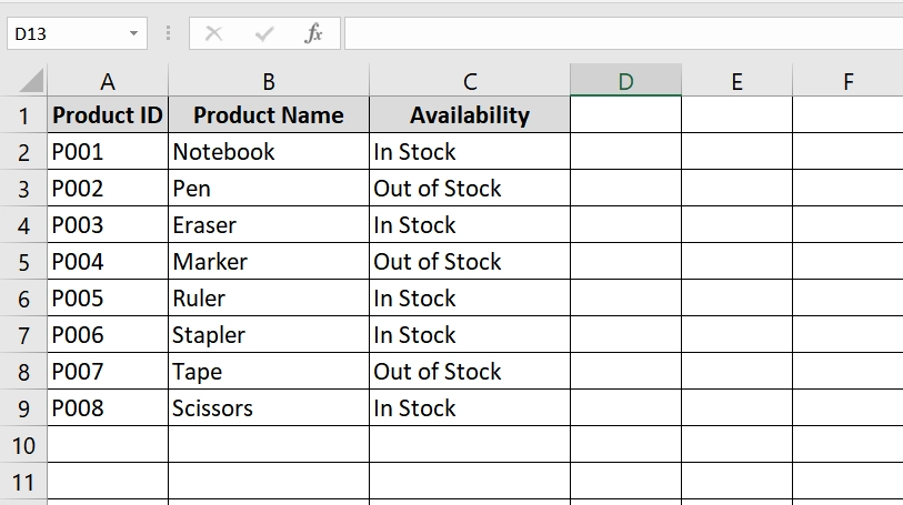
➤ Open your dataset that has a clear header row (e.g., A1:C1) and values underneath. In our case:
- Range = A1:C9
- Headers = Product ID, Product Name, Availability
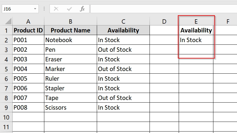
➤ Copy the header of the column you want to filter (e.g., “Availability“) to a separate cell, e.g., E1.
➤ Under it (E2), type the filter value: In Stock
Now, E1:E2 becomes your criteria range.
➤ Select any cell in your data range (A1).
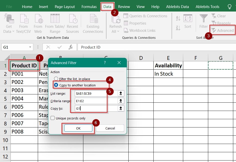
➤ Go to the Data tab > Click Advanced (in the Sort & Filter group).
➤ In the Advanced Filter dialog box:
- Choose “Copy to another location”
- List range: A1:C9
- Criteria range: E1:E2
- Copy to: Choose a new range like G1 (or any blank part of the sheet)
- Click OK.
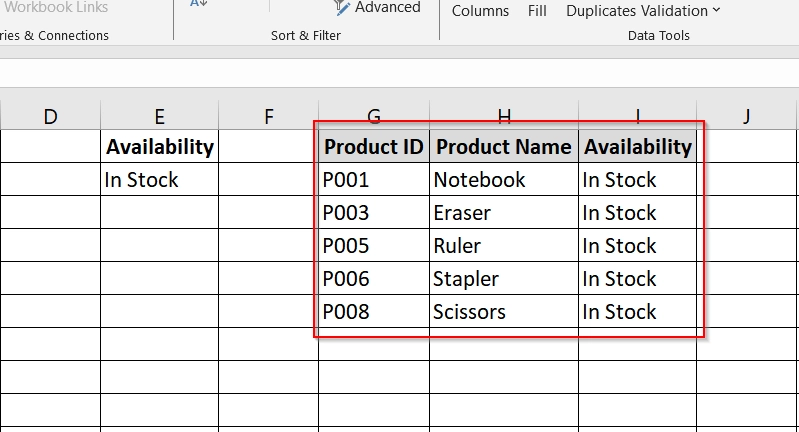
➤ You’ll see only the “In Stock” rows copied to the new location starting from G1.
Notes:
➧ The original dataset remains untouched until you manually delete it.
➧ You can use multiple criteria by expanding the criteria range (e.g., filtering by both “Availability” and “Product Name”).
Frequently Asked Questions (FAQs)
Why can’t I delete all filtered rows at once?
If you select the entire range, Excel may include hidden rows. That’s why, delete only the visible (filtered) row.
What’s the difference between Delete and Clear Contents?
“Delete” removes the entire row from the worksheet. “Clear Contents” removes the data but keeps the row structure intact.
Can I use keyboard shortcuts to delete filtered rows?
Yes. After selecting visible filtered rows, press Ctrl + – (minus) and choose Shift cells up to delete properly.
Concluding Words
Deleting filtered rows in Excel is always a useful technique for cleaning up data. We have shown 4 easy to use methods. If you want to remove outdated records, null values, or any other conditionally filtered rows, you can use any of these methods.