Pulling data from another sheet based on specific criteria is a common task that helps in consolidating, analyzing, and summarizing information efficiently. Excel offers several methods using functions like VLOOKUP, INDEX/MATCH, FILTER, and advanced techniques using Power Query that allow you to dynamically extract data matching your conditions from other sheets.
In this article, you’ll learn step-by-step how to use each method to pull matching data from a different sheet based on single or multiple criteria.
Steps to pull data from another sheet based on criteria in Excel:
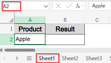
➤ Go to your target sheet (Sheet1), and place your lookup value in A2 (e.g., “Apple”).
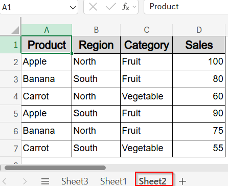
➤ In Sheet2, make sure the value you’re trying to look up (Product) is in the first column of the data range.
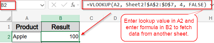
➤ Click into cell B2 in Sheet1 (where you want the pulled Sales value to appear).
➤ Enter the formula: =VLOOKUP(A2, Sheet2!$A$2:$D$7, 4, FALSE)
➤ Press Enter. It will return the first matching Sales value for “Apple” in Sheet2.
Retrieve Value with VLOOKUP Function (Single Criteria)
VLOOKUP is one of the most widely used formulas to retrieve data from another sheet when you have a unique identifier or key to match. It works well for simple lookups where you need the first matching value from a table.
Steps:
➤ Go to your target sheet (Sheet1), and place your lookup value in A2 (e.g., “Apple”).
➤ In Sheet2, make sure the value you’re trying to look up (Product) is in the first column of the data range.

➤ Click into cell B2 in Sheet1 (where you want the pulled Sales value to appear).
➤ Enter the formula:
=VLOOKUP(A2, Sheet2!$A$2:$D$7, 4, FALSE)
This searches for the value in A2 (“Apple“) in the first column of the Sheet2 range (A2:A7), and pulls the corresponding value from the 4th column (Sales).
➤ Press Enter. It will return the first matching Sales value for “Apple” in Sheet2.
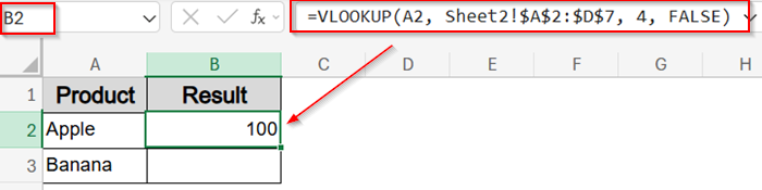
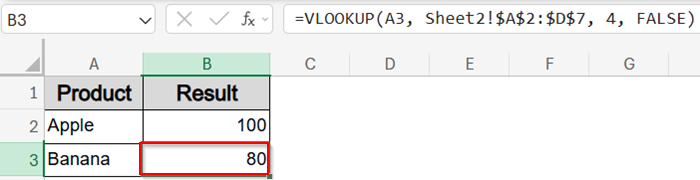
➤ Use the AutoFill handle to pull the Sales value for additional lookup values like Banana which is 80.
Match Two Criteria Using INDEX-MATCH Formula
The INDEX/MATCH function is more flexible than the VLOOKUP function as it allows leftward lookups and can be combined with multiple criteria for advanced data retrieval.
Steps:
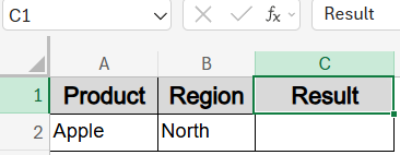
➤ In Sheet1, ensure A2 contains the Product (e.g., “Apple“) and B2 contains the Region (e.g., “North“).
➤ In Sheet2, the source table should have Product in column A, Region in column B, and Sales in column D.

➤ Click in C2 of Sheet1 (where you want the pulled Sales).
➤ Enter the array formula:
=INDEX(Sheet2!$D$2:$D$7, MATCH(1, (Sheet2!$A$2:$A$7=A2)*(Sheet2!$B$2:$B$7=B2), 0))
This finds the row where both Product and Region match your inputs, and returns the corresponding Sales value from column D.
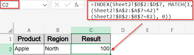
➤ In older Excel versions, press Ctrl + Shift + Enter . In Excel 365, just hit Enter.
Pull All Matching Rows with FILTER Function (Excel 365)
The FILTER function returns all rows from another sheet that meet one or more conditions. It’s available for modern Excel versions and updates automatically when data changes.
Steps:
➤ In Sheet1, ensure column A contains the Product (e.g., “Apple“, “Carrot”) and column B contains the Region (e.g., “North“, “South”).
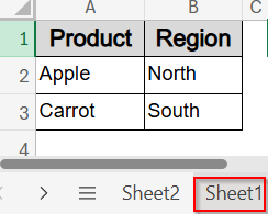
➤ In Sheet2, the source table should have Product in column A, Region in column B, and Sales in column D.

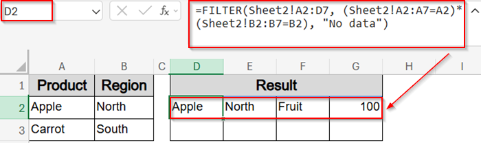
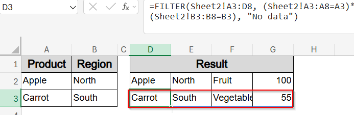
➤ Go to Sheet1, and in cell D2, enter the following formula:
=FILTER(Sheet2!A2:D7, (Sheet2!A2:A7=A2)*(Sheet2!B2:B7=B2), “No data”)
This filters Sheet2 to return rows where both Product and Region match Sheet1’s A2 and B2.
➤ Press Enter. All columns (Product to Sales) for matching entries will appear starting in D2.
➤ Use the AutoFill handle to get matching values for Carrot from South starting from D3 cell.
Pull Data with XLOOKUP Function
XLOOKUP is a modern and flexible function. It simplifies lookups and replaces older functions like VLOOKUP and INDEX/MATCH. It supports exact matches, handles errors efficiently and also allows searching in any direction.
Steps:
➤ In Sheet1, ensure A2 contains the Product (e.g., “Apple“) and B2 contains the Region (e.g., “North“).

➤ In Sheet2, the source table should have Product in column A, Region in column B, and Sales in column D.
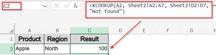
➤ Go to Sheet1, and click in cell C2.
➤ Enter the formula:
=XLOOKUP(A2, Sheet2!A2:A7, Sheet2!D2:D7, “Not found”)
This looks for the Product in A2, searches it in Sheet2 column A, and returns the corresponding value from column D (Sales).
➤ Press Enter. It will return the Sales value for the first matching Product.
Note:
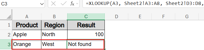
XLOOKUP handles errors with “Not found” and doesn’t require sorting or remembering column numbers.
Get Filtered Data Using Power Query
Power Query is a powerful tool for importing, transforming, and filtering data from different sheets or even external sources without complex formulas. It suits large datasets and repetitive tasks.
Steps:
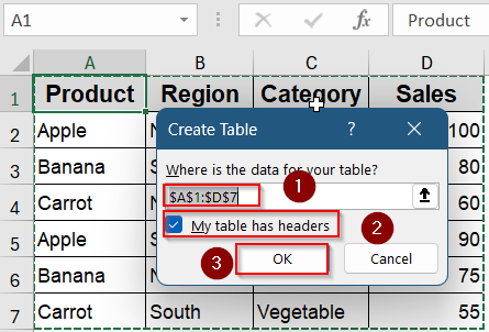
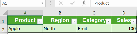
➤ In Sheet2, convert your data range to a table:
➤ Select range A1:D7 >> press Ctrl + T >> Check your headers and click OK.
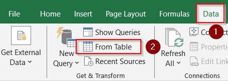
➤ Go to the Data tab >> click From Table/Range.
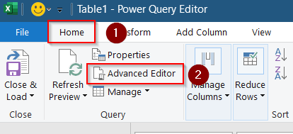
➤ When Power Query Editor opens, click the Home tab >> Advanced Editor.
➤ Modify the query to include a filter like this:
let
    Source = Excel.CurrentWorkbook(){[Name="Table1"]}[Content],
    FilteredRows = Table.SelectRows(Source, each ([Product] = "Apple" and [Region] = "North"))
in
    FilteredRows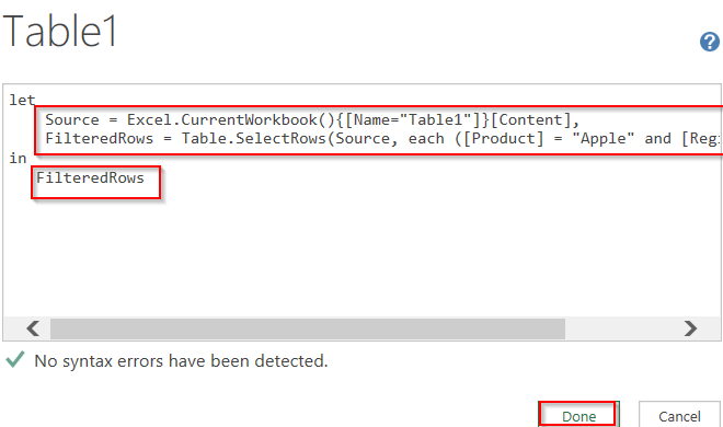
➤ Click Done.
➤ Click Close & Load to output results on a new sheet.
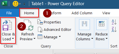
This filters the dataset where Product is “Apple” and Region is “North” and loads it to your sheet.
Frequently Asked Questions
Can I pull data from a closed workbook based on criteria?
No, formulas with VLOOKUP or FILTER function require the source workbook to be open; however, Power Query can connect to closed workbooks and extract data dynamically.
How do I handle multiple criteria in data retrieval formulas?
Combine criteria with multiplication * inside MATCH or use the FILTER function with logical conditions for simple multi-criteria lookups and filtering.
Is it possible to pull data dynamically as the source data updates?
Yes, formulas like FILTER and INDEX/MATCH update automatically when source data changes. On the other hand, Power Query requires manual refresh to update pulled data.
What if no matching data is found during lookup?
Use IFERROR or the third argument in FILTER function to display a friendly message or blank instead of errors when no data matches the criteria.
Wrapping Up
In this tutorial, we explored multiple methods to pull data from another sheet in Excel based on criteria from classic options like VLOOKUP and INDEX/MATCH function to modern and dynamic ones like XLOOKUP, FILTER, and Power Query. Each method serves a unique purpose, depending on your Excel version, the number of conditions, and whether you prefer formulas or UI-based filtering. Feel free to download the practice file and share your feedback.