Sometimes in Excel, you need to pull more than one result. For example, a customer may appear several times in a sales record, and you want to list all of their order amounts. In these cases, Excel’s lookup functions can help you return multiple values quickly.
There are several ways to look up multiple values using Excel formulas. You can return each match in separate cells, group them into a single text result, or filter them based on one or more conditions. It depends on your Excel version and the method you choose.
In this article, you’ll learn how to look up multiple values in Excel using functions like FILTER, TEXTJOIN, IF, TRUE, and XLOOKUP. Each method is designed for a specific task, so you can choose the one that works best for your dataset.
Here’s how to look up multiple values in Excel by combining the TEXTJOIN function and IF statement in one cell:
➤ Open your dataset in Excel.
➤ Click on cell G2 and enter the following formula:
=TEXTJOIN(“, “, TRUE, IF(A:A=F2, D:D, “”))
➤ If you’re using Excel 365 or 2019, press Enter.
➤ If you’re using Excel 2016 or earlier, press Ctrl + Shift + Enter to make it an array formula.
➤ Excel will return a single text string containing all the order amounts for Alice, separated by commas.
➤ Now, drag the fill handle down to copy the formula to the rest of the rows for Bob, David, and Charlie.
Use the FILTER Function to Return All Matching Values
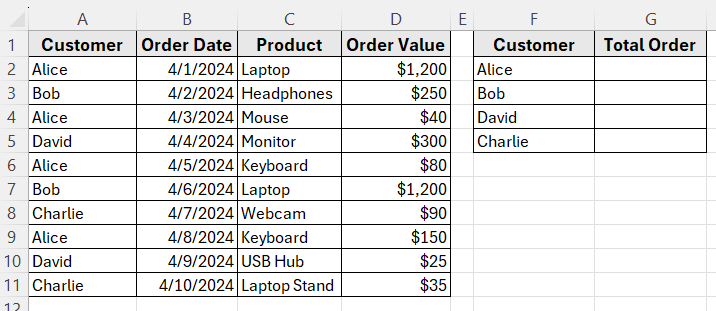
In the following dataset, we have a simple customer order log that tracks purchases over time. Column A lists the Customer Names, Column B shows the Order Dates, Column C contains the Product Names, and Column D holds the Order Values.
On the right, we’ve created a lookup table with Customer Names in Column F. Our goal is to retrieve all the Total Order Amount each customer has ordered and display them in Column G next to their name.
We’ll use this dataset to demonstrate multiple methods to look up and return all matching values for a specific customer name in Excel.
The FILTER function is the easiest way to look up multiple values and return all matching results. It works only in Excel 365 or Excel 2021 and is perfect when you want to extract several values that meet the same condition.
In this method, we’ll pull all the order amounts placed by a single customer from our dataset.
Let’s find all orders made by Alice.
Here’s how to do it:
➤ Open your dataset in Excel.
➤ Click on cell G2, enter the following formula
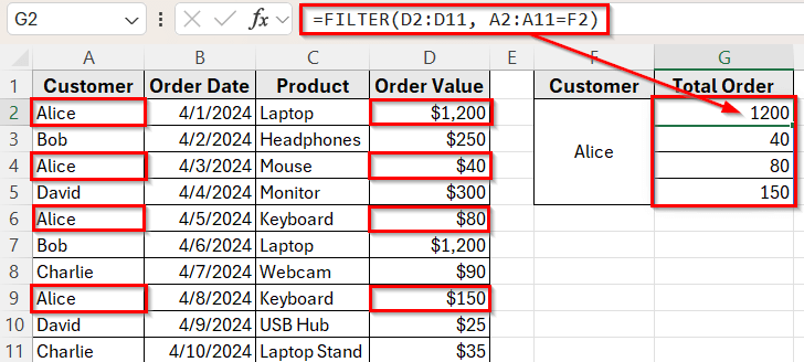
=FILTER(D2:D11, A2:A11=F2)
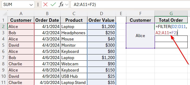
➤ Press Enter. You’ll instantly see all the order amounts for Alice spill into cells below G2.
This formula works dynamically. If you change the name in F2 to Bob or David, the results will update automatically to show their orders.
➤ Now, drag the fill handle down to copy the formula to the rest of the rows for Bob, David, and Charlie.

Note:
The FILTER function is only available in Excel 365 and Excel 2021. If you’re using an older version of Excel, try the next method which works with array formulas.
Combine TEXTJOIN with IF to Return Multiple Values in One Cell
If you want to look up multiple matching values and display them in a single cell, you can use the TEXTJOIN function combined with an IF statement. This is useful when you don’t need the results to appear in separate rows, but still want to see all the matches together.
This method works in Excel 365 and Excel 2019. If you’re using Excel 2016 or earlier, you’ll need to enter it as an array formula using Ctrl + Shift + Enter .
Let’s use this method to return all Total Order Amounts for a selected customer, like Alice.
Here’s how to apply this method:
➤ Open your dataset in Excel.
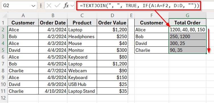
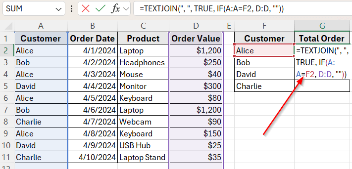
➤ Click on cell G2 and enter the following formula:
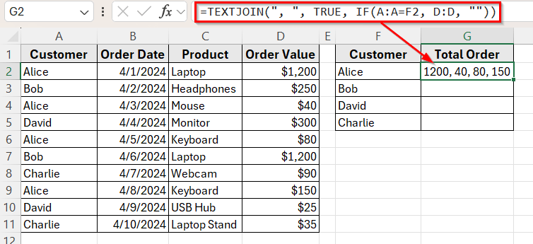
=TEXTJOIN(", ", TRUE, IF(A:A=F2, D:D, ""))
➤ If you’re using Excel 365 or 2019, press Enter.
➤ If you’re using Excel 2016 or earlier, press Ctrl + Shift + Enter to make it an array formula.
➤ Excel will return a single text string containing all the order amounts for Alice, separated by commas.
Note:
This method returns a text value, not numbers. That means you won’t be able to use the result directly in calculations unless you split and convert it back into numbers.
Use XLOOKUP with Multiple Lookup Values
The XLOOKUP function is one of Excel’s most flexible lookup tools. It allows you to look up multiple values at once and return either one or several results based on your dataset.
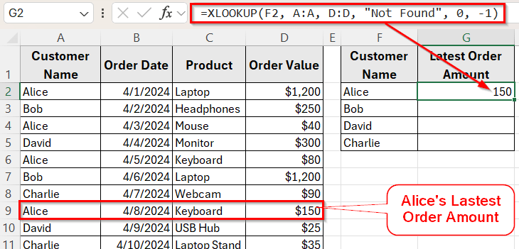
In this method, we’ll look up multiple customer names at the same time and return their corresponding latest order amounts. We’ll retrieve the most recent order for four customers: Alice, Bob, David and Charlie.
Here’s how to do it:
➤ Open your dataset in Excel and select the column where you want to display the latest order amount of Alice.
➤ In cell G2, enter the following formula
=XLOOKUP(F2, A:A, D:D, "Not Found", 0, -1)
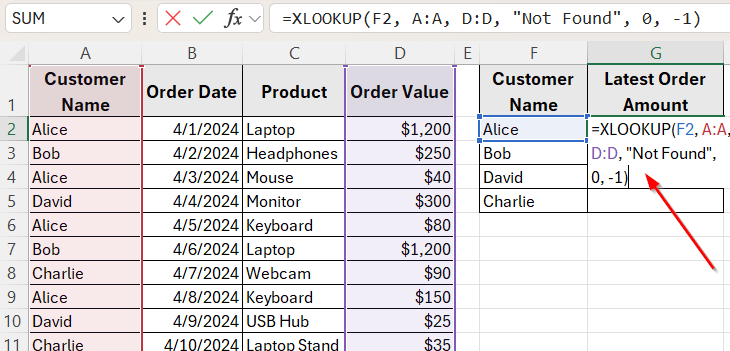
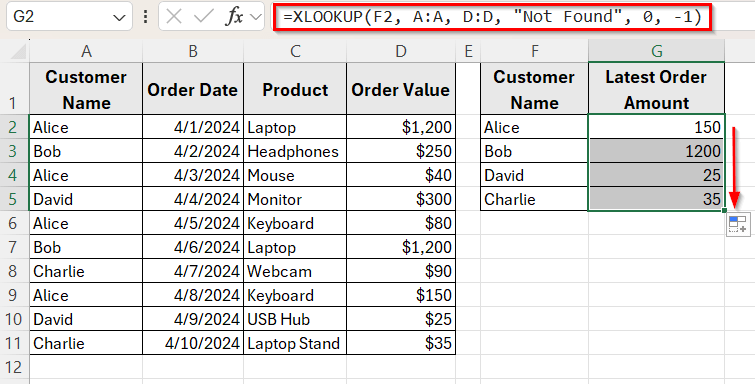
➤ Press Enter, then drag the fill handle down to apply the formula to the rest of the rows.
➤ Next, drag the fill handle down to copy the formula to the rest of the rows for Bob, David, and Charlie.
Note:
This method works best when each lookup value has one latest record or when you only need one result per name. If you want all matching results instead of just the latest one, use the FILTER method we covered earlier.
Lookup Multiple Values with Multiple Criteria Using FILTER
Sometimes you need to search based on more than one condition. For example, you might want to find all order amounts for a specific customer for a specific product. When you have multiple criteria, the FILTER function can handle it smoothly.
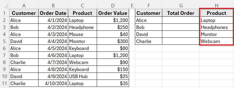
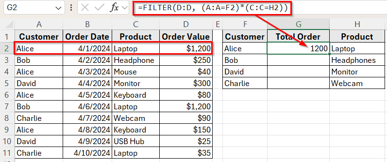
In this method, we’ll look up values based on both Customer Name and Product. To do that, we’ll first add a column for Product Name to complete our dataset. Then we’ll find all order amounts for Alice for the product Laptop.
Here’s how to apply this method:
➤ First, add product names in Column H. For example, type Laptop in cell H2, Headphones in H3, Monitor in H4, and Webcam in H5.
➤ Click on cell G2 and enter this formula
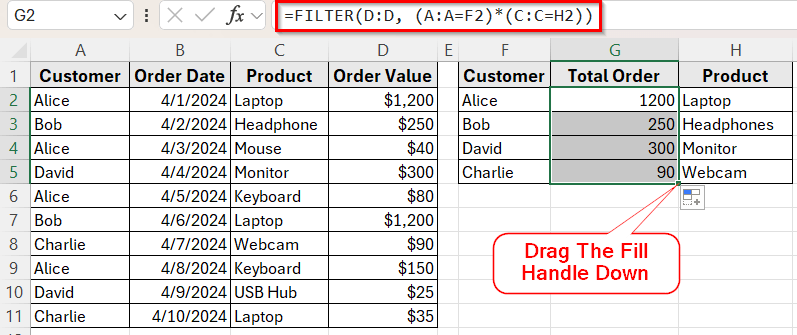
=FILTER(D:D, (A:A=F2)*(C:C=H2))
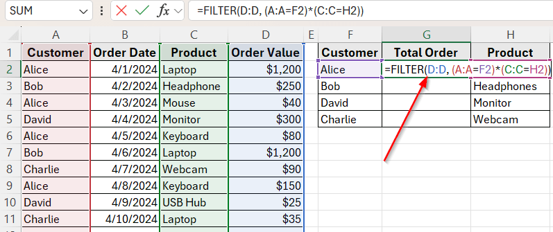
➤ Press Enter. You’ll see all order amounts that match both the customer name and the product.
➤ Drag the fill handle down to cell H5 to copy the formula for the rest of the rows.
Note:
The FILTER function only works in Excel 365 or Excel 2021. For earlier versions of Excel, this kind of multi-criteria filtering requires helper columns or array formulas.
Frequently Asked Questions
How do I look up multiple values at once in Excel?
You can use functions like FILTER, XLOOKUP, or TEXTJOIN with IF statements to look up multiple values based on a list or multiple criteria. These methods allow you to return all matching records or just the most recent match, depending on your needs.
Can I return all matching results in one cell?
Yes. You can use the TEXTJOIN function with an IF statement to combine all matching results into a single text string. This method is useful when you want to display multiple values together in one cell, separated by commas.
Wrapping Up
Excel provides several useful ways to look up multiple values. You can use Excel built-in functions depending on your Excel version and what kind of result you want.
To return all matching results, the FILTER function works best. If you only need to get one matching value, XLOOKUP, TEXTJOIN and IF functions can handle it well.
Each method works best in different situations. Pick the one that matches your needs. These lookup techniques will help you manage and analyze your data more efficiently in Excel.