Copying a cell format really helps when you’re changing fonts, adding borders, setting up colors, and adjusting cell sizes all at once in Google Sheets. Sometimes, it’s time consuming to get everything looking just right to do it all manually. Having to repeat that same formatting for other cells, rows, or entire sections. It can be a real headache.
However, Google Sheets has a few built-in tools that let you copy formatting from one cell to another in just a couple of clicks. In this guide, we’ll learn how to copy formatting in Google Sheets using a few different methods.
If you want to copy format in Google sheet, it is the easiest and most commonly used method. Follow the below steps:
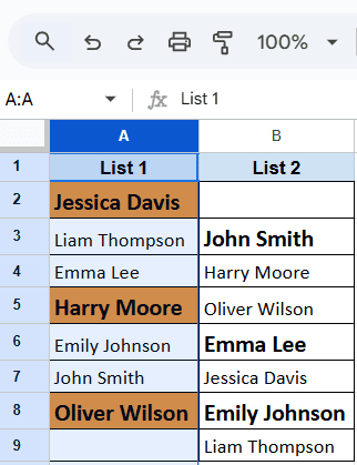
➤ First, select the cell or column with the formatting you want to copy. For example, we select Column A.
➤ Click the column header to select the entire column format.
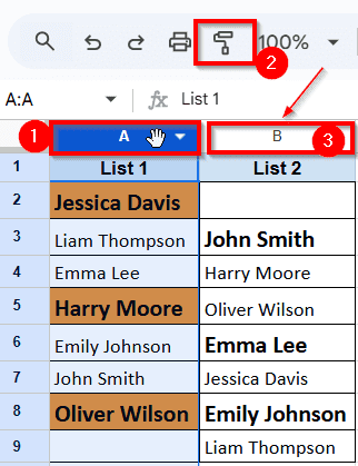
➤ When the selected area turns blue, click the Paint format icon. It looks like a paint roller and right below the menu section.
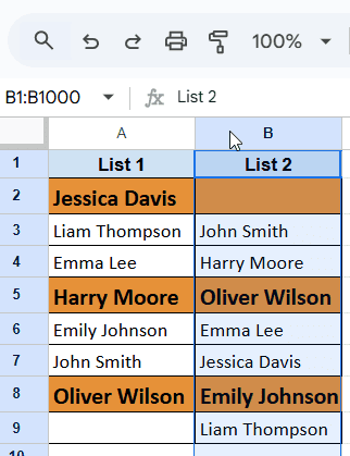
➤ Now click the column header, where you want to apply the same formatting. Here we click Column B to successfully copy the exact format of Column A.

What Does Copying a Format Mean in Google Sheets?
In Google Sheets, copying a cell format or formatting means duplicating the exact style of a cell, or even an entire row or column, without copying its content. Instead of manually repeating all those steps for other cells, you can just copy the formatting and paste it wherever you need.
Here’s what copying format can include:
- Font type and size
- Text color and background color
- Bold, italic, or underline
- Borders and alignment
- Number formatting like currency, percentage, etc.
Use Format Painter Tool
Usually, the most used and easiest method to copy format in Google Sheet is using the Format Painter Tool. Just follow the below steps:
➤Select the cell or column with the formatting you want to copy. For example, we select Column A.
➤Click the column header to select the entire column format.
➤ When the selected area turns blue, click the Paint format icon. It looks like a paint roller and right below the menu section.
➤ Now click the column header, where you want to apply the same formatting. Here we click Column B to successfully copy the exact format of Column A.
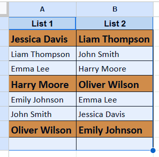
That’s how you can copy format from any cells, rows or columns to another, without changing the actual content.
Apply Copy and Paste Special Features
If you want to copy the format of multiple rows and columns at once, this method is the other easiest way to go. This method is perfect when you’re working across different sheets or applying consistent formatting to large sections without affecting the content.
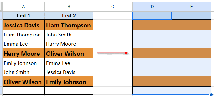
➤ First, you have to select the entire section or a range of cells. For example, in the image below, we want to copy the format of Column A and Column B.
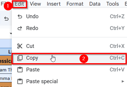
➤ Next, go to the top menu and click on the Edit option and a drop-down menu will appear.
➤ Click on Copy to copy the entire format of the selected cells.
➤ Now, select the cell or range where you want to apply the copied formatting. In this case, we’re selecting a blank cell as the starting point.
➤ Click on the Edit menu again, and this time, you’ll see the Paste option in the drop-down.
➤ Hover your cursor over the Past Special option and this will open another side menu.
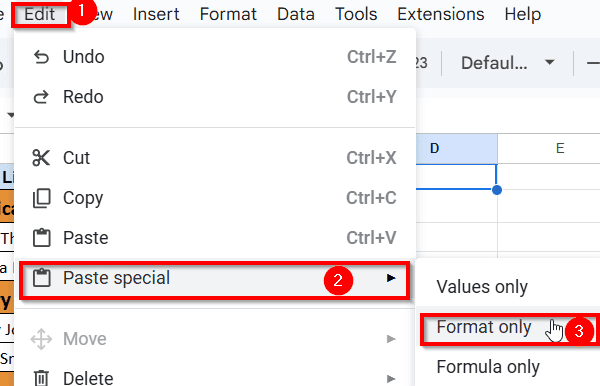
➤ Click on Format only option from the side menu, and the formatting will be applied to your selected cells.
Frequently Asked Questions
How do I duplicate formatting in Google Sheets?
To duplicate formatting in Google Sheets, you can use the Paint Format tool. It looks like a little paint roller at the top of the page.
Here’s how:
➤ First, click on the cell that has the look you want to copy.
➤ Then click the Paint Format icon.
➤ Now, click on the cell where you want to apply that same look.
➤ The new cell will instantly match the formatting of the original one.
How do I auto format in Google Sheets?
Here’s a simple way to auto format in Google Sheets:
➤ First, highlight the group of cells you want to auto format. For example, from A1 to A100.
➤ Then go to the top menu and click on Format, and choose Conditional formatting from the list from the drop down menu.
➤ A panel will open on the right side. From the drop-down menu, choose Custom formula if you want to set your own rule.
➤ Now enter your condition. For example, if you want to highlight rows where the value in Column A is over 100, you can write a formula like =A1>100.
➤ After that, choose how you want those cells to look, maybe a green background or bold text.
➤ Once you’re happy with the style, click Done.
How do I fix the format in Google Sheets?
To fix formatting in Google Sheets:
➤ Open your sheet and select the cells you want to adjust.
➤ Click Format from the top menu.
➤ Choose from options like bold, text color, alignment, cell background, or number format.
➤ Changes apply instantly, making your data look clean and organized.
Concluding Words
Copy formatting in Google Sheets can save you time and help keep your spreadsheet looking clean and consistent. If you’re working with a few cells or large sections, using tools like Paint Format or Paste special makes the process easy.
Once you get the hang of it, you’ll spend less time on manual formatting and more time focusing on your actual data. Try out the different methods mentioned and use the one that fits your workflow best. Google Sheets gives you the flexibility you just need to know where to look.