
There are several reasons to hide unused cells in Google Sheets. You may find the infinite rows and columns distracting while working. Or you don’t want unwanted edits in unused areas. Knowing how to hide unused cells in Google Sheets keeps your data clean and helps the sheet load faster. Though Google Sheets doesn’t have a method to hide specific cells. However, you can hide rows and columns. There are some simple methods to do that easily.
Suppose we want to hide the unused cells on the right side of our data in Google Sheets. So we need to hide the columns next to the data cells. Follow the steps below to do that.
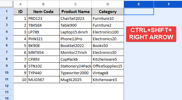
➤ Select the column name first.
➤ Press Ctrl + Shift + Right Arrow at the same time.
➤ All the columns next to the data will be selected.
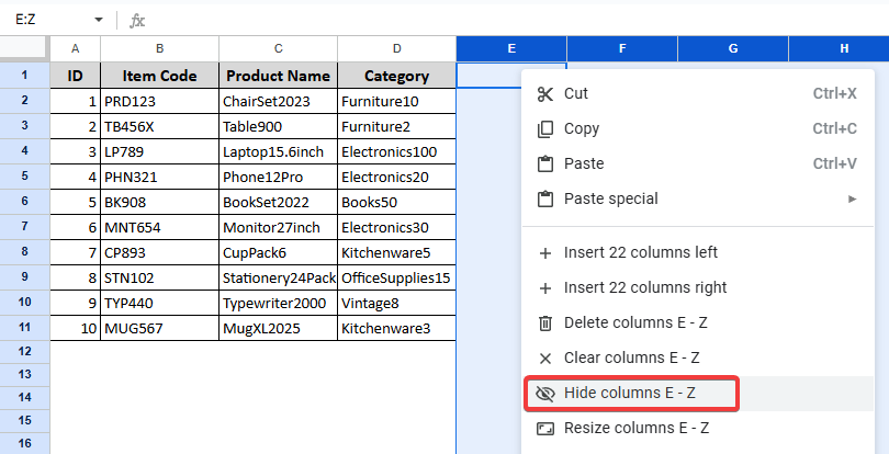
➤ Right-click on the mouse, and the context menu will appear.
➤ Select “Hide columns E-Z” to hide selected columns.

What Are Unused Cells in Google Sheets?
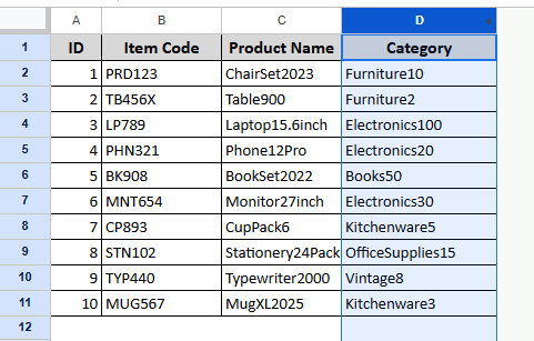
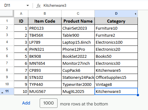
The cells that don’t contain any data are referred to as unused cells. It also means the blank rows and columns outside the data range.
In this article, we will guide you to hide unused cells (rows or columns) in Google Sheets. We will discuss four different methods of how to hide unused cells in Google Sheets. We will hide unused cells using a simple keyboard shortcut, the context menu, Google Apps Scripts and Group action.
Using Keyboard Shortcut to Hide Unused Cells
You can easily hide the unused cells using a simple keyboard shortcut. There are two shortcuts to hide unused cells in Google Sheets. One is for hiding unused columns, and another one is for hiding unused rows.
Hiding Unused Rows
Steps:
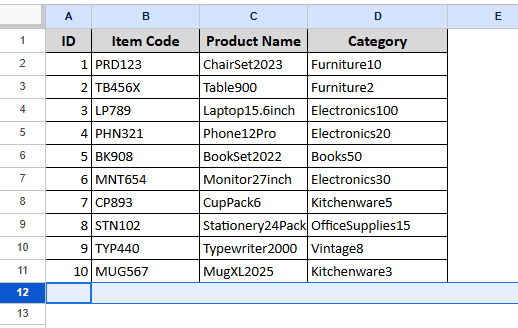
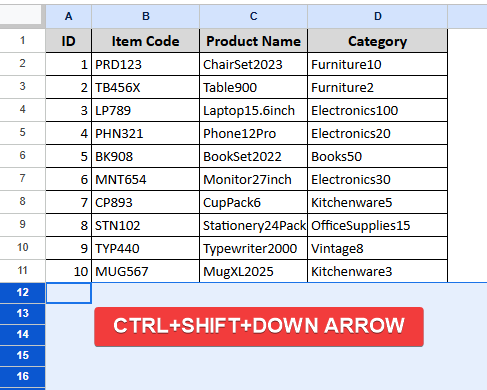
➤ Click on the row number first.

➤ Press Ctrl + Shift + Down Arrow to select all the rows below. It will select all the unused rows below.

➤ Press Ctrl + Alt + 9 to hide the unused rows.
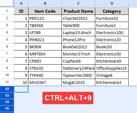
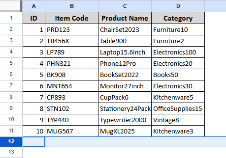
The rows are hidden, as shown in the following image.
Hiding Unused Columns
Steps:
➤ Select the first unused column name.
➤ Press Ctrl + Shift + Right Arrow to select all the columns to the right.
➤ Press Ctrl + Alt + 0 to hide all the unused columns.
Using the Context Menu Options to Hide Unused Cells
The most common practice for hiding unused cells in Google Sheets is to use the context menu. You can hide both columns and rows using the context menu.
Hiding Unused Rows
Steps:
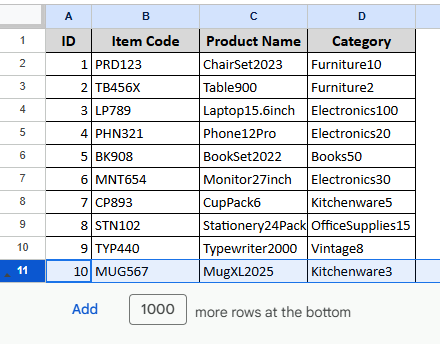
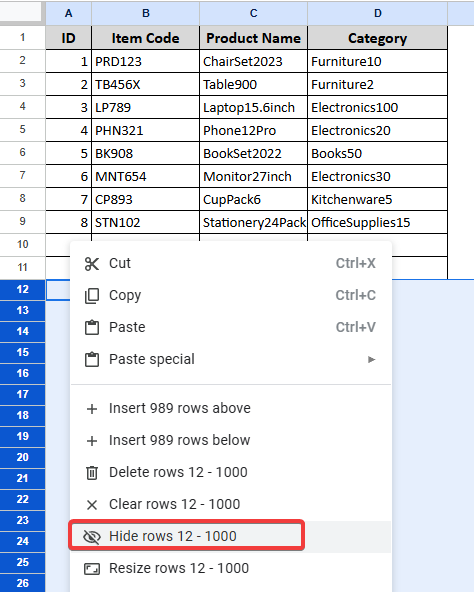
➤ Select the first unused row number.
➤ Press Ctrl + Shift + Down Arrow at the same time to select all the blank rows below.

All the rows below the data will be selected.
➤ Right-click on the mouse, and the context menu will appear.
➤ Select “Hide columns 12 – 1000” to hide selected columns.
Hiding Unused Columns
Steps:
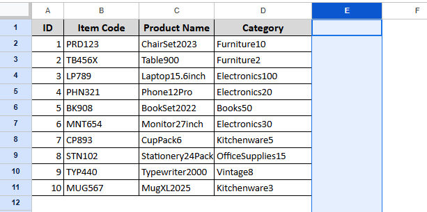
➤ Select the column name first.
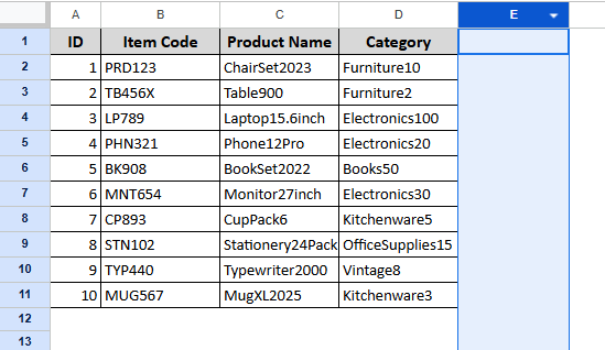
➤ Press Ctrl + Shift + Right Arrow at the same time to select all the blank columns.

➤ All the columns next to the data will be selected.
➤ Right-click on the mouse, and the context menu will appear
➤ Select “Hide columns E-Z” to hide selected columns.
Using Google Apps Script
Another dynamic solution to hide unused cells is to use Google Apps Script. If you want to hide unused cells in a sheet that you update regularly. You can apply the following method.
Steps:
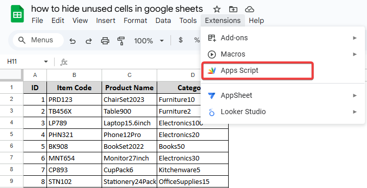
➤ Go to the Extensions menu bar in Google Sheets.
➤ Select Apps Script. It will open a code editor.
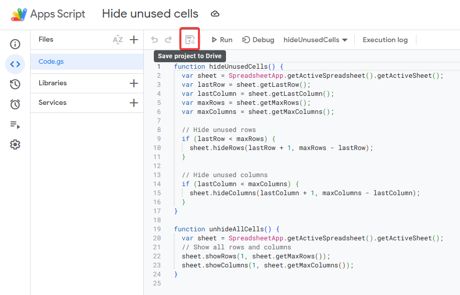
➤ Delete any code in the editor, then paste the script below.
function hideUnusedCells() {
var sheet = SpreadsheetApp.getActiveSpreadsheet().getActiveSheet();
var lastRow = sheet.getLastRow();
var lastColumn = sheet.getLastColumn();
var maxRows = sheet.getMaxRows();
var maxColumns = sheet.getMaxColumns();
// Hide unused rows
if (lastRow < maxRows) {
sheet.hideRows(lastRow + 1, maxRows - lastRow);
}
// Hide unused columns
if (lastColumn < maxColumns) {
sheet.hideColumns(lastColumn + 1, maxColumns - lastColumn);
}
}
function unhideAllCells() {
var sheet = SpreadsheetApp.getActiveSpreadsheet().getActiveSheet();
// Show all rows and columns
in the sheet.showRows(1, sheet.getMaxRows());
sheet.showColumns(1, sheet.getMaxColumns());
}
➤ Click on the Save icon to save the project to Drive. (Give it a name like “Hide Unused Cells”).
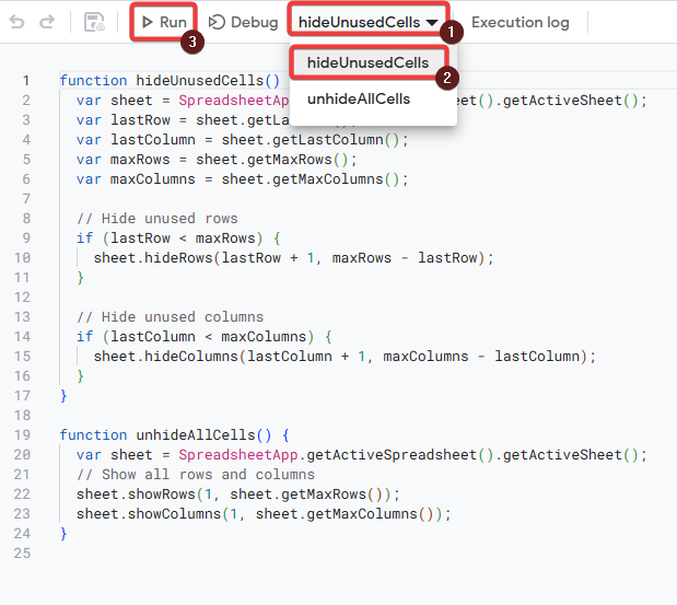
➤ Select the hideUnusedCells() option from the dropdown.
➤ Click on the Run icon.
➤ You’ll need to authorize permissions the first time.
➤ To reverse, run unhideAllCells().
Hiding Rows or Columns as a Group
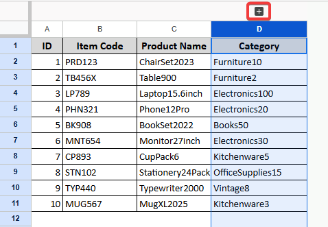
You can hide unused cells as a group, also. In this way, you can hide and unhide the cells with just one click on the minus or plus icon.
Hide Rows as Group
Steps:
➤ Click on the row number first.
➤ Press Ctrl + Shift + Down Arrow to select all the rows below.
It will select all the unused rows below.
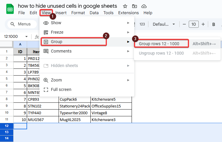
➤ Select View >> Group >> Group rows 12 – 1000.
➤ You can also group the rows from the context menu.
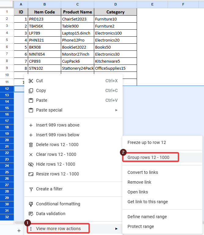
➤ You can also group the rows using the Shift + Alt + Down Arrow Arrow shortcut.
➤ You will see a minus (-) icon to the left.
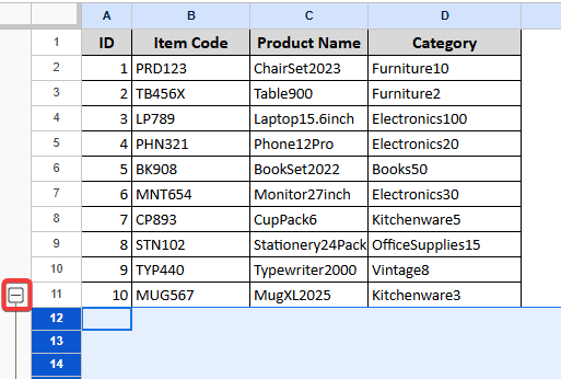
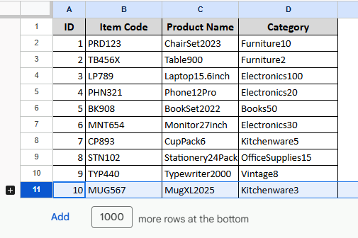
➤ Click on the minus icon, and you will see it hides all the rows below.
Hide Columns as Group
Steps:
➤ Select the first unused column name.

➤ Press Ctrl + Shift + Right Arrow to select all the columns to the right.

This will select all the columns to the left of the dataset.
➤ Select View >> Group >> Group columns E-Z
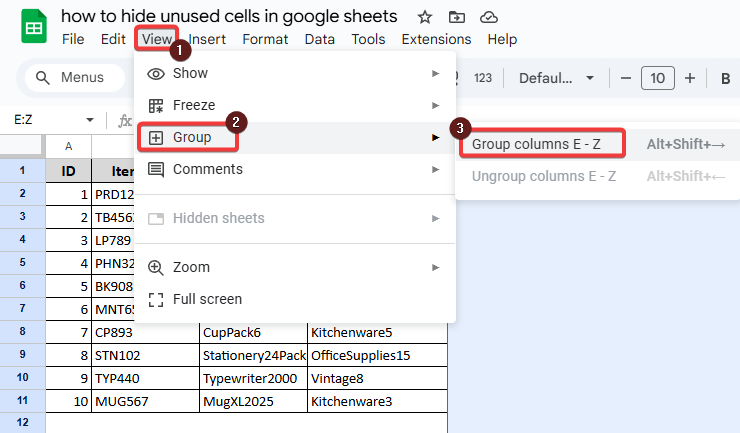
➤ You will see a minus (-) icon above.
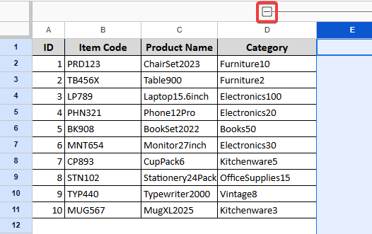
➤ Click on the minus icon, and you will see it hides all the columns to the right of it.
Frequently Asked Questions (FAQs)
If I hide rows or columns, will the data be deleted?
No. Hiding only alters the display. All hidden cells still exist, and you can easily unhide.
Can I use conditional formatting to hide empty cells?
No. Conditional formatting only changes appearance (color, font, etc.). It can’t actually hide rows or columns.
Can I hide individual cells (not whole rows or columns) in Google Sheets?
Unfortunately no. There is no option to hide an individual cell in Google Sheets till now. You can only hide a whole row or column in Google Sheets.
Wrapping Up
While Google Sheets doesn’t support hiding specific unused cells, it has the option to hide rows and columns. Hope this article will help you tidy up your sheet. Whether you have a sheet full of budget, records, or any kind of data.
You can choose manual hiding for quick cleanups or automating via Apps Script. It will help you to keep only the relevant data in view. It helps you to focus, share cleaner sheets, and avoid unnecessary scrolling.