
When you need to show data from one sheet to another sheet, you need to link the two sheets in Google Sheets. Your time will be saved because you don’t need to copy and paste the data when changes are made. When you change any data in the main sheet, the corresponding values in the other sheet will be updated automatically if the two sheets are linked. In this article, we will explore all the methods to link two sheets in Google Sheets.
If you want to change or update your sales data in the sales data sheet, the stock data sheet will be updated automatically by linking the two sheets. To link two sheets in Google Sheets, you need to follow these steps:
➤ Go to another sheet.
➤ Click cell C2 and type.
=IF(A2=””,””, SUMIF(‘Sales Data’!B: B, A2, ‘Sales Data’!C: C))
➤ Press Enter, and you will see the sold quantity is updated and linked in this new sheet.
In this article, we will learn how to link two sheets in Google Sheets using various methods. Using the SUMIF function, QUERY & VLOOKUP functions, and a pivot table are the methods to link two sheets in Google Sheets.
Linking Two Sheets & Auto-Updating Data Based on Calculations
When you modify any information in one sheet, the other sheet will be updated automatically because the two sheets are linked. One sheet can “look up” or “pull” data from another sheet based on calculations.
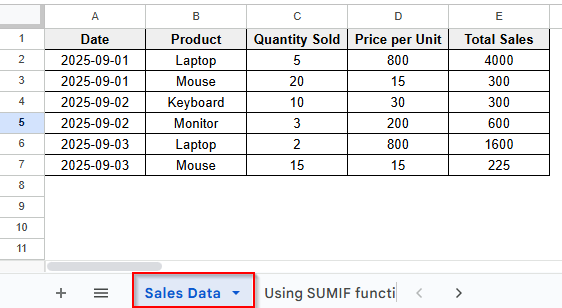
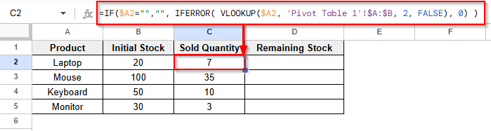
Let’s examine the dataset below, which includes a sales data sheet with various values, such as price, quantity sold, price per unit, and total sales. In another sheet, there are stock updates in the stock data sheet. The amount sold will be automatically updated by calculating the total quantity sold. After that, we can count the remaining stock by subtracting the amount sold from the initial stock.
Steps:
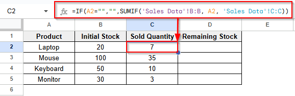
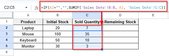
➤ In another sheet, which is named “1. Using SUMIF Function”, in cell C2, write this formula
=IF(A2="","",SUMIF('Sales Data'!B:B, A2, 'Sales Data'!C:C))
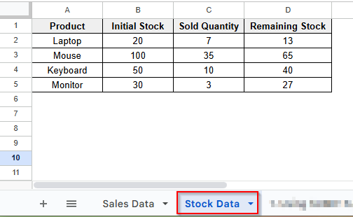
➤ Press Enter, and you will see that the first data is calculated from the main sheet, and it is “7”. Drag the formula down to see the other result.
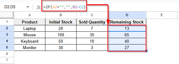
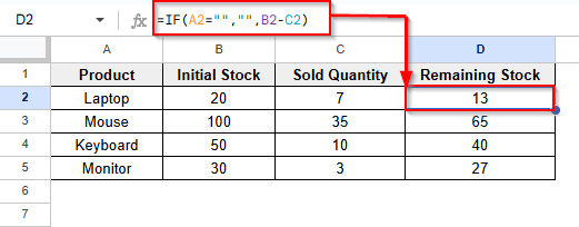
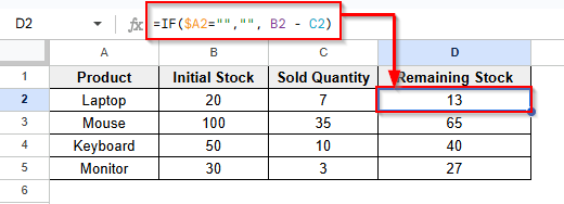
➤ To see the remaining stock, click on cell D2 and write this formula, and Press Enter, and see the first result is 13. Drag down and see the other result.
=IF(A2="","",B2-C2)
Using the QUERY & VLOOKUP Functions
In this method, we will use the QUERY & VLOOKUP functions to link two sheets. The QUERY function will create a sales data summary table. Then, using the VLOOKUP function, we can find the sold quantity and remaining stock data.
Steps:
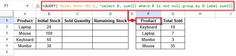
➤ Click on cell F2 and write this formula to create a summary table from the sales data sheet.
=QUERY('Sales Data'!B1:C, "select B, sum(C) where B is not null group by B label sum(C) 'Total Sold'", 1)
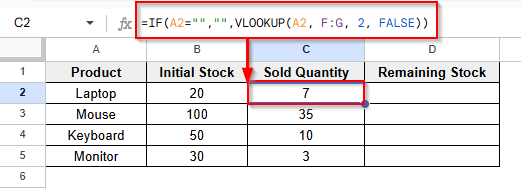
➤ Click on cell C2 and write this formula
=IF(A2="","",VLOOKUP(A2, F:G, 2, FALSE))
➤ Then drag cells to see other results.
➤ Click on cell D2 and write this formula
=IF(A2="","",B2-C2)
➤ Then drag cells to see other results.
Using Pivot Table for Linking Two Worksheets
By creating a pivot table in another sheet, we can link two sheets in Google Sheets. The pivot table is a summary of the total quantity sold of the product. Then we can find the remaining stock of the updated data.
Steps:
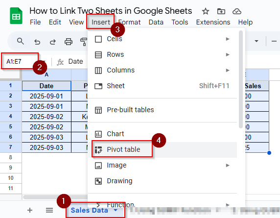
➤ In the sales data sheet, select A1:E7, then click Insert > Pivot Table
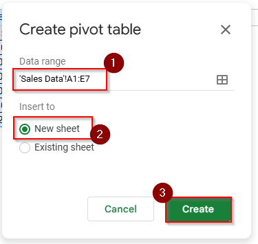
A pop-up window will come, select data range A1:E7, choose a new sheet and click the create button.
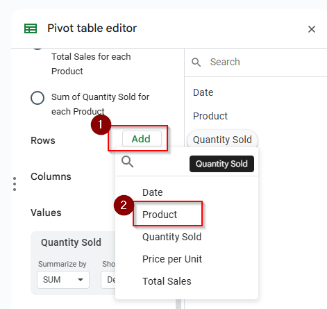
➤ In the pivot table editor, add rows and choose the product to show product data in the rows.
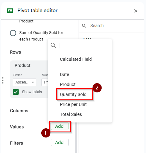
➤ Then add the quantity sold values in the pivot table editor.
➤ Now the pivot table is created with the sheet name “pivot table 1”.
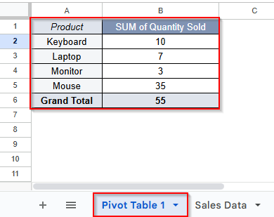
➤ Click on cell C2 and write this formula to see the sold quantity data.
=IF($A2="","", IFERROR( VLOOKUP($A2, 'Pivot Table 1'!$A:$B, 2, FALSE), 0) )
➤ Then drag down to see other results.
➤ Click on cell D2 and write this formula to see the remaining stock data.
=IF($A2="","", B2 - C2)
➤ Then drag down to see other results.
Frequently Asked Questions(FAQs)
Is it possible to link an entire sheet without selecting a specific range?
No, you need to select a specific cell range (e.g., A1:E11) to link an entire sheet. Without selecting the cell range, it’s not possible to link any sheet.
If I make any changes to the source sheet, will the linked data update automatically?
Yes, if you change anything in the main sheet, all the changes will be updated in the linked sheet automatically and instantly.
Is it possible to link formatting (colors, fonts, borders) along with values in the linked sheet?
No, it’s not possible. Formatting will not be linked in the linked sheet. Only values from the source sheet will be linked in another sheet.
What will happen if the source file is deleted, or I lose access?
The linked sheet will show #REF! or #N/A errors. To fix this issue, you need to keep a backup of the source file.
Concluding Words
In this article, we learned how to link two sheets in Google Sheets and update automatically using the SUMIF, QUERY & VLOOKUP functions and using the pivot table. If you change any data in the sales data sheet, then the other sheet will automatically be updated. Feel free to give us suggestions and feedback regarding this article.