If you’re organizing priority lists, and sorting tasks by status or sizes of products Google Sheets lets you customize your sort order according to real-world needs, not just alphabetically. With clearer and more purposeful data through sorting, you can make better decisions and attain better representation.
This article will walk you through with 3 simple & effective methods to apply custom sorting using built-in features and formulas.
Steps to custom sort in easy ways:
➤ Use the SORT function for single or multiple columns.
=SORT(Range, Column, true) or
=SORT(Range, Col 1, true, Col 2, false)
➤ You can use the built-in SORT RANGE option from the option menu.
➤ Use the ARRAY function to set specific order.
=SORT (RANGE, ARRAYFORMULA (MATCH (COLUMN,{DATA ORDER},0)),true)
Note:
Here ‘SORT’, ‘MATCH’, and ‘ARRAYFORMULA’ are functions to perform sorting. Again, ‘true’ is marked as a boolean value for A-Z /ascending order and ‘false’ for Z-A / descending order.
Sorting Single Column with 'Sort Range' Option
If you need to sort the values in one column without shifting the rest of your data, using the Sort range option in Google Sheets can be a perfect approach. This method keeps data intact as it controls how a single column appears, either in ascending or descending order.
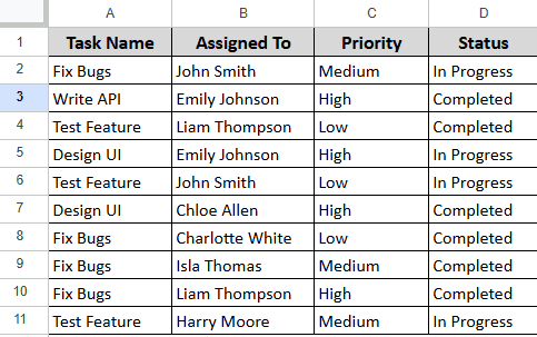
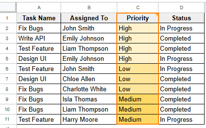
Here’s a sample dataset related to task statements and progress. Any of the columns or multiple columns can be sorted to a desired column or order. We’ll simply follow the Sort range option from the Context Menu options to custom-sort a single column easily.
Steps:
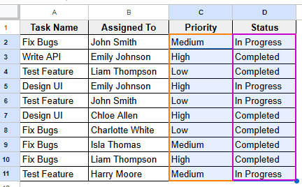
➤ Select the range for a single column C.
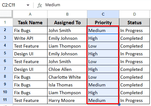
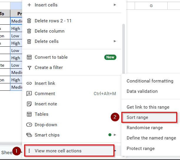
➤ Open Context Menu by right-clicking your mouse.
➤ Then go to View More Cell Actions > Sort Range.
➤ A Pop-up as ‘Sort Range from C2 to C11’ will appear where you have to choose the Ascending or Descending Order.
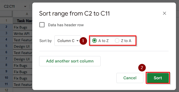
➤ If you have ‘Header Row’, choose Data Has Header Row > select desired header Priority from Sort By: > choose Ascending or Descending Order > then click Sort.
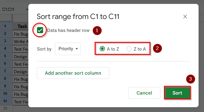
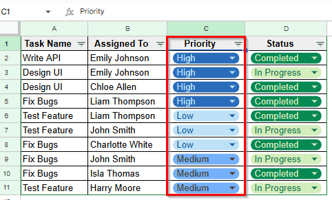
➤ Your existing dataset will be sorted based on Column C as shown here.
Sorting Multiple Columns with Sort Range from the Menu Bar
Using the Sort Range option from the Menu Bar makes it easier to sort data in multiple columns. It’s explained here how to sort data across several columns for clear and structured results.
It helps keep your spreadsheet organized and easy to analyze, especially when prioritizing specific data groups.
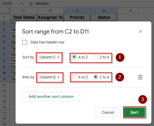
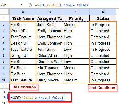
➤ After selecting Column C and D, select Data from the Menu Bar > click Sort Range > select Advanced Range Sorting Options.
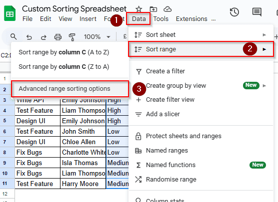
➤ Select Add another sort column to add Column D.
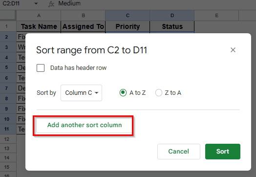
➤ After adding Column D, choose order A-Z or Z-A according to your need and click the Sort button.
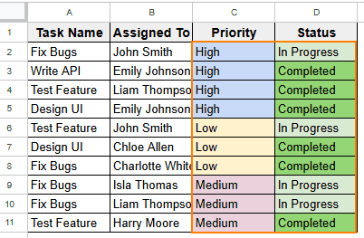
➤ Then sorted Dataset will be shown as a result.
Sorting Multiple Columns with SORT Function
Sorting more than one column in need is easy in Google Sheets. This section walks you through how to sort data across multiple columns using the SORT function. It will give you clear and structured results.
It also keeps a spreadsheet easy to read and analyze prioritizing data or data groups.
Steps:
➤ Select a blank cell A14.
➤ Now specifying range A2 to D12 and column C to be sorted, write the formula:
=SORT (A2:D12, C2:C12, true)
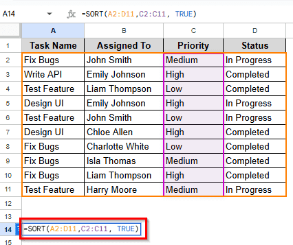
➤ Press Enter to achieve sorting which will be shown as a separate table.
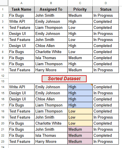
➤ In case of sorting multiple columns under different conditions, write the formula:
=SORT (A2:D11, 1, true, 4, false)
Note:
Here the dataset is sorted by Task Name and then by the descending order of Status.
➤ Press Enter for the sorted results.
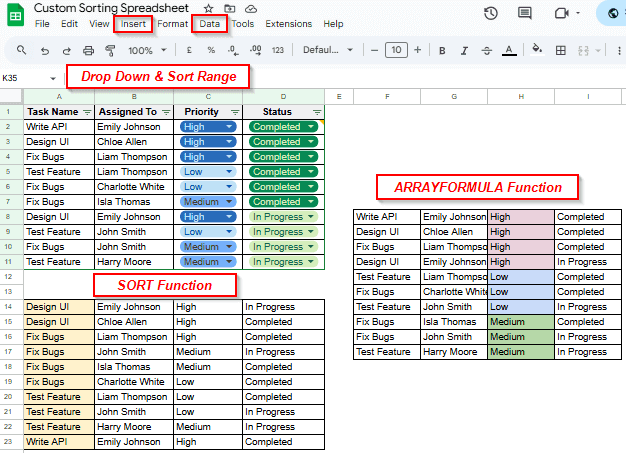
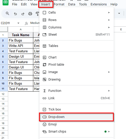
Custom Sorting Order Using Drop Down & Filter
This is a smart way to deal with dynamic datasets and obviously saves you time and hassle.
➤ Select the columns C and D for sorting.
➤ Then follow these simple steps: Insert > Drop Down.
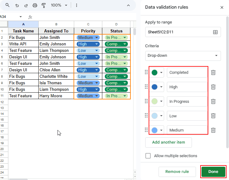
➤ Now the result shows a Data Validation Rules Box. It allows you to apply rules like customizing the Drop Downs.
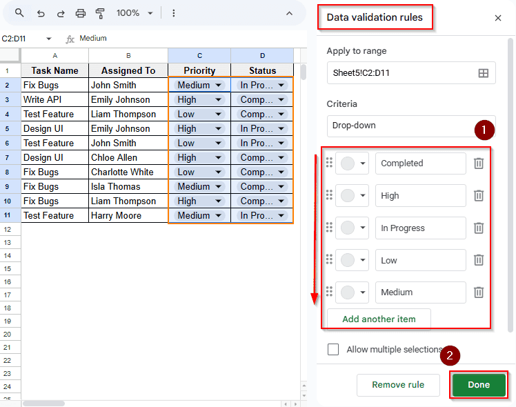
➤ Press Done to see the results.
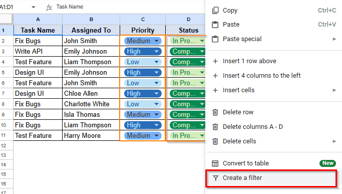
➤ Select the Header Row > access the Options Menu > choose Create a Filter.
➤ Now select the Filter Icon from header of column C, Priority to sort according to your choice.
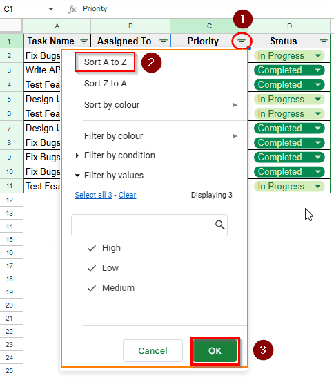
➤ The results will show after clicking the OK button. Here the dataset is sorted alphabetically by ascending order (A-Z).
Sorting in Specific Order Using ARRAYFORMULA Function
Arranging data in a custom or specific order saves time and enhances clarity while working with large datasets. Now we’ll show how to sort values automatically based on a defined sequence using the ARRAYFORMULA function in Google Sheets.
Steps:
➤ Select a blank cell A14 to write the formula.
➤ Specify RANGE and Column to be sorted, and use the formula:
=S0RT(RANGE, ARRAYFORMULA(data range, MATCH(desired column, {”Medium”, ”Low”,“High”}, 0), true))
Note:
The function ARRAYFORMULA specifies that multiple calculations on various items are to be performed in the array, and MATCH function returns the relative position of an item in an array or cell range.
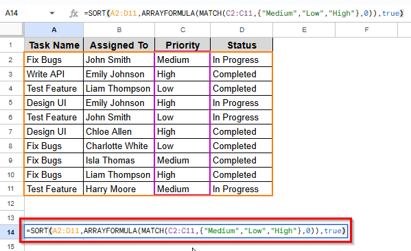
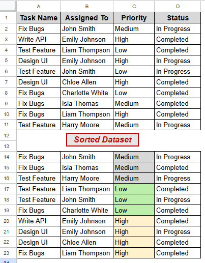
➤ Now press Enter to have sorted results as a separate dataset.
Frequently Asked Questions
Can I sort data arranged horizontally?
Yes, you can. And doing that is simple with the TRANSPOSE function. Use this formula:
=SORT (TRANSPOSE(Cell Range), Row Range, true)
Does Sorting occur automatically in Google Sheets?
Yes, it automatically changes every time you add or adjust any data in the original dataset. This is because the sorted table is a dynamic table that keeps up with the updates.
How to find the SORT function from the Toolbar?
The easiest way is to follow this order of actions: Insert > Function > Filter > Sort.
Wrapping Up
In this article, we’ve learned how to apply custom sorting in Google Sheets using the SORT function on single or multiple columns and based on different conditions. Additionally, it showed us easy ways of using built-in features of Sort Range from the Options Menu and SORT from Insert or Data in the menu bar. Feel free to try these techniques yourself, and share your valuable feedback or suggestions.