
Creating a master sheet can be helpful when you’re working with a spreadsheet full of data spread across multiple tabs. If you manage different regional or departmental sheets, it can be hard to get a full picture of all your data. Instead of checking each tab separately, you can use a few simple methods to build a master sheet that combines everything into one place.
In this article, we’ll show you how to make a master sheet in Google Sheets using easy techniques that will save time and keep your data organized.
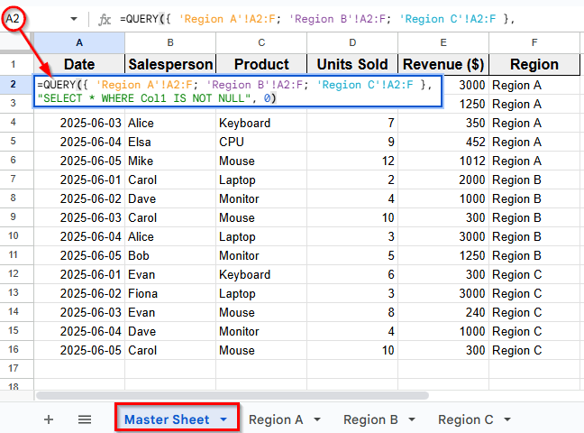
Here’s how to use QUERY function to make a Master Sheet in Google Sheets:
➤ Open your Google Sheets file and go to the Master Sheet.
➤ Click on cell A2, and enter the following formula to pull data from Region A, Region B, and Region C together.
=QUERY({ ‘Region A’!A2:F; ‘Region B’!A2:F; ‘Region C’!A2:F }, “SELECT * WHERE Col1 IS NOT NULL”, 0)
➤ Press Enter.
➤ This formula combines the data ranges from all three sheets. You’ll see the Master Sheet now collects all data from Region A, B, and C.
Setting Up All Source Sheets First in Google Sheets
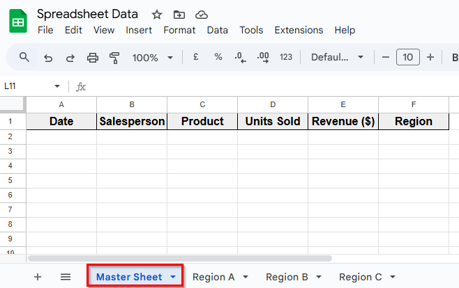
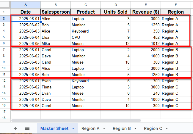
In the following dataset, there are four sheets labeled Master Sheet, Region A, Region B, and Region C. Each regional sheet contains similar types of data, including Date, Salesperson, Product, Units Sold, Revenue, and Region. These sheets are already organized with headers and sample entries.
We’ll use this setup to apply and practice the methods for combining data into a single Master Sheet in Google Sheets.
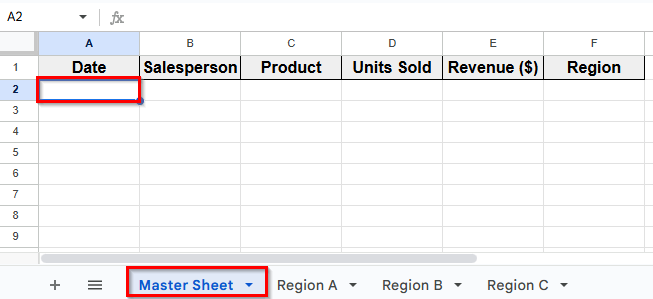
Here is the Master Sheet:
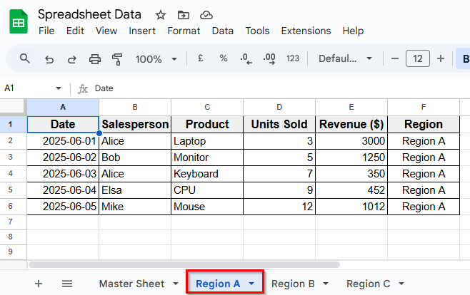
Here is the Region A sheet:
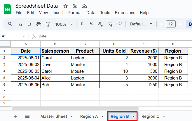
Here is the Region B sheet:
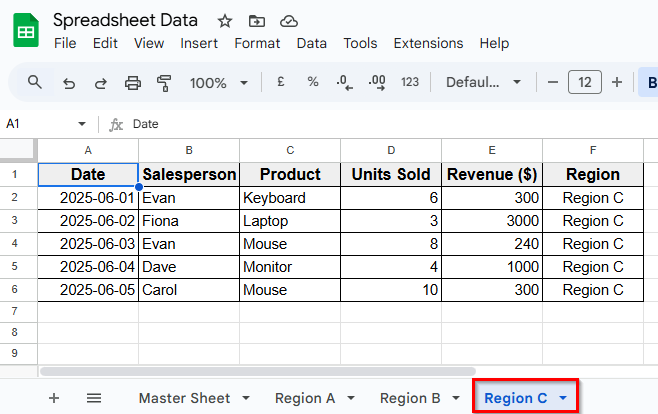
And here is the Region C sheet:
FILTER Function to Pull Data Automatically to the Master Sheet
If you want your master sheet to update automatically when the original sheets are updated, you can use the FILTER function.
Step 1: Manually Collect Data One by One from Each Region
Here’s how to apply this method:
➤ Open your Google Sheets and go to the Master Sheet and select cell A2.
➤ In cell A2, enter the formula below to pull data from Region A
=FILTER('Region A'!A2:F, LEN('Region A'!A2:A))
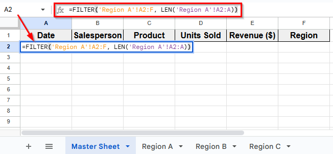
➤ Press Enter.
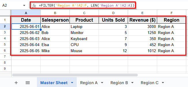
➤ This formula imports all the filled rows from Region A into the Master Sheet, skipping any blank ones.
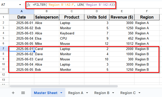
➤ Next, move to cell A7, and enter a similar formula for Region B
=FILTER('Region B'!A2:F, LEN('Region B'!A2:A))
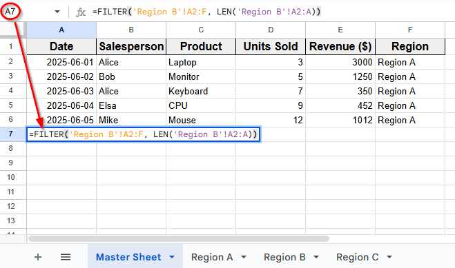
➤ Press Enter.
➤ Now, you’ll see all the data of Region B’s data appear directly below Region A’s data in the Master Sheet.
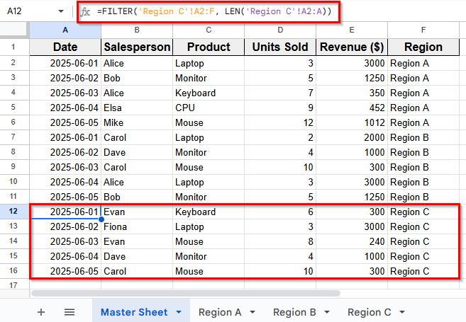
➤ Finally, go to cell A12, and enter this formula for Region C
=FILTER('Region C'!A2:F, LEN('Region C'!A2:A))
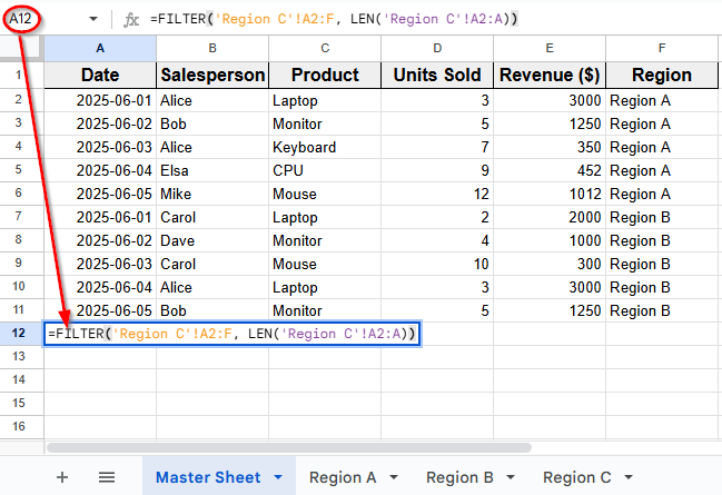
➤ Press Enter.
➤ This method automatically updates your Master Sheet with the data of Region C.
➤ Now, your Master Sheet automatically collects data from all regional sheets, and it will update in real time as those sheets change.
Step 2: Combine FILTER Functions Inside Curly Braces to Collect All Data At Once
Instead of entering separate formulas for each region, you can combine them all in one formula using brackets {}. This method arranges all the filtered results together.
Here’s how to do it:
➤ From the Master Sheet select cell A2.
➤ Enter this combined formula
={FILTER('Region A'!A2:F, LEN('Region A'!A2:A));FILTER('Region B'!A2:F, LEN('Region B'!A2:A));FILTER('Region C'!A2:F, LEN('Region C'!A2:A))}
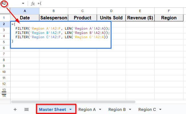
➤ Press Enter.
➤ This formula pulls filled rows from all three regions (Region A, Region B, and Region C) and combines them into the Master Sheet automatically and in real time.
Using QUERY Function to Combine All Sheets
Another simple way to bring data from multiple sheets into a Master Sheet is by using the QUERY function. Unlike FILTER, the QUERY function lets you pull and customize data in the Master Sheet.
Here’s how to use this method:
➤ Open your Google Sheets file and go to the Master Sheet.
➤ Click on cell A2, and enter the following formula to pull data from Region A, Region B, and Region C together.
=QUERY({ 'Region A'!A2:F; 'Region B'!A2:F; 'Region C'!A2:F }, "SELECT * WHERE Col1 IS NOT NULL", 0)
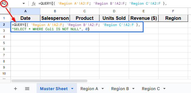
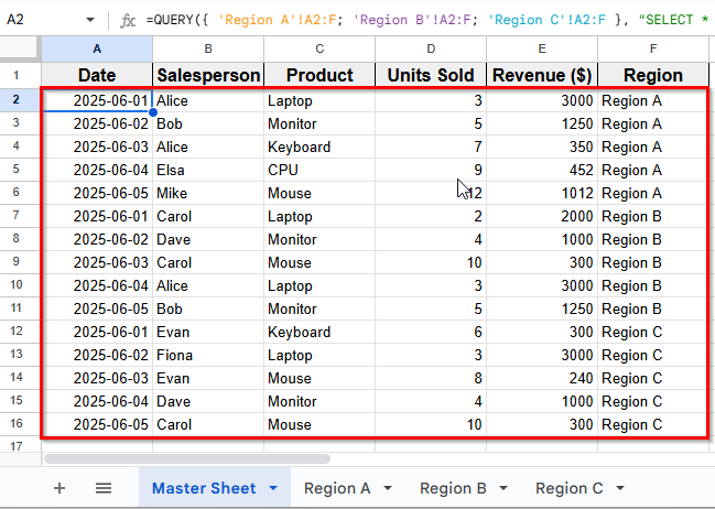
➤ Press Enter.
➤ This formula combines the data ranges from all three sheets. You’ll see the Master Sheet now collects all data from Region A, B, and C.
Using IMPORTRANGE Function for Different Google Sheets Files
If your regional data is stored in different Google Sheets files instead of separate tabs, you can use the IMPORTRANGE function to pull the data into your Master Sheet.
Here’s how to apply this method:
➤ Open your Google sheets file and go to the Master Sheet where you want to bring all data together.
➤ In cell A2, enter the following formula to import data from an external sheet. This example is for Region A
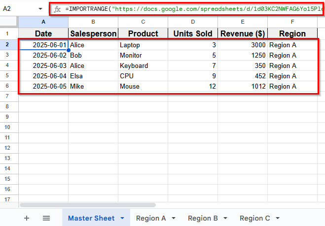
=IMPORTRANGE("https://docs.google.com/spreadsheets/d/1d03KC2NWFAG6Yo15PleW-M6C9ghxytvyBSD0jMQpe_8/edit?usp=sharing", "Region A!A2:F")
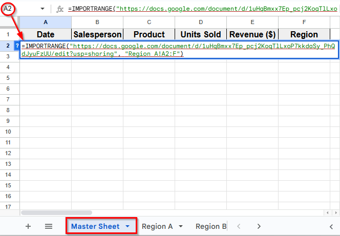
➤ Replace “Spreadsheet_URL” with the actual URL or ID of the external spreadsheet that contains the Region A data.
➤ Now the data from Region A will appear in your Master Sheet automatically.
➤ Repeat the same process to collect data from Region B and Region C. If they are in different Google Sheets files, update the spreadsheet URL and sheet name, then apply the formula in the rows below.
Frequently Asked Questions
What is a Master Sheet in Google Sheets?
A master sheet is a single tab that collects and displays data from multiple other sheets. This central sheet makes it easier to view everything in one place. It also ensures updates from other sheets appear automatically.
How do I create a master sheet in Google Sheets?
You can create a master sheet by pulling data from other sheets using functions like FILTER, QUERY, or IMPORTRANGE. These formulas help collect and organize data from different sheets into one central sheet.
How to merge data from different Google Sheets into one master sheet?
With the IMPORTRANGE function, you can connect and pull data from other Google Sheets files. Just use the spreadsheet URL and sheet range in your formula to collect data in the Master sheet.
Wrapping Up
If you’re working with different sheets for various teams, locations, or projects, a Master Sheet helps you bring all your data together. Instead of manually checking each tab, you can use formulas like FILTER, QUERY, or IMPORTRANGE to combine everything into a single, organized view.
Choose the method that best fits your needs. With a master sheet, your workflow will be more efficient, and your reporting process will become much easier to manage.

