A moving average is a useful way to spot patterns in your data. It shows the average over a set number of days, helping you see trends more clearly by smoothing out small changes.
In trading and other data analysis tasks, moving averages are often used to understand the price direction over time. They are a common part of tools used to study past performance and make better decisions.
You can use a moving average in Google Sheets to track stock prices, sales, website traffic, or temperature readings. It’s quick to set up and works well with time-based data.
In this guide, you’ll learn how to calculate a moving average in Google Sheets step by step using some simple formulas.
The ARRAYFORMULA function helps you apply a formula to an entire column without copying it down manually.
Here’s how to apply this method:
➤ Open your dataset in the Google Sheets.
➤ Click on cell C4, where you want the moving averages to start.
➤ Enter the following formula =ARRAYFORMULA(IF(ROW(B4:B16)-ROW(B4)+1<=ROWS(B2:B16)-2, (B2:B14 + B3:B15 + B4:B16)/3, “”))
➤ Press Enter.
➤ Now Column C will automatically show the 3-day simple moving average, starting from row 4 down to row 16.
What is the Simple Moving Average (SMA)?
The Simple Moving Average (SMA) is a way to find the average value of data over a number of days.
For example, if you have sales numbers for 3 days, the SMA adds those 3 numbers together and divides them by 3. The result is the average for that period. As you move down the list, the average updates to include the next group of days.
This helps smooth out daily ups and downs, so you can focus on the overall trend.
SMA is often used to track things like stock prices or daily sales. It gives a clear view of how your numbers are changing over time.
For example, we have have these numbers for 3 days:
Day-1 = 120, Day-2 = 150, and Day-3 =180
To find the 3-day simple moving average: (120 + 150 + 180) / 3 = 150
Now, for the next 3-day period (Day 2 to Day 4), you use the next set of values.
Applying AVERAGE Function To Calculate Moving Average
In the following dataset, we take a random trading list that shows daily sales figures for the first 15 days of June 2025. There are three columns labeled Date, Sales ($), and 3-Days SMA. Column A includes the dates, Column B shows the sales data recorded each day, and Column C is currently empty.
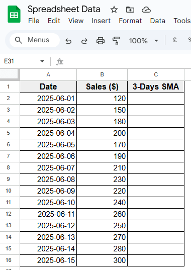
We’ll use this third column to calculate the 3-day simple moving average using different formulas in Google Sheets.
The AVERAGE function is the simplest way to calculate a moving average in Google Sheets. It works by taking a group of values and returning their average. In this example, we’ll use it to calculate a 3-day simple moving average based on the sales data.
To apply this method, follow these steps:
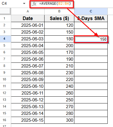
➤ Open your dataset in Google Sheets.
➤ Select Column C to display the 3-days simple moving average.
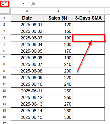
➤ Click on cell C4, since the first 3 values are in B2 to B4.
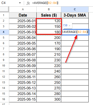
➤ Type this formula:
=AVERAGE(B2:B4)
➤ Press Enter.
➤ The result will be the average of the first three sales values. For example:
(120 + 150 + 180) / 3 = 150
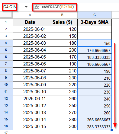
➤ Now, click on the bottom-right corner of the cell and drag it down through the rest of Column C to apply the same logic for the remaining dates.
Using the ARRAYFORMULA Function
The ARRAYFORMULA function helps you apply a formula to an entire column without copying it down manually. When calculating a moving average, it’s a good choice for automating results, especially if your data grows over time.
We’ll use ARRAYFORMULA in combination with a row-wise calculation that manually averages three consecutive cells.
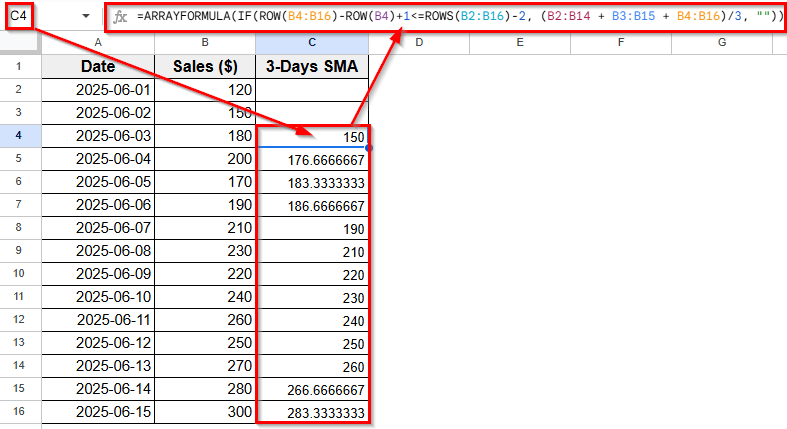
Here’s how to apply this method:
➤ Open your dataset in the Google Sheets.
➤ Click on cell C4, where you want the moving averages to start.
➤ Enter the following formula
=ARRAYFORMULA(IF(ROW(B4:B16)-ROW(B4)+1<=ROWS(B2:B16)-2, (B2:B14 + B3:B15 + B4:B16)/3, ""))
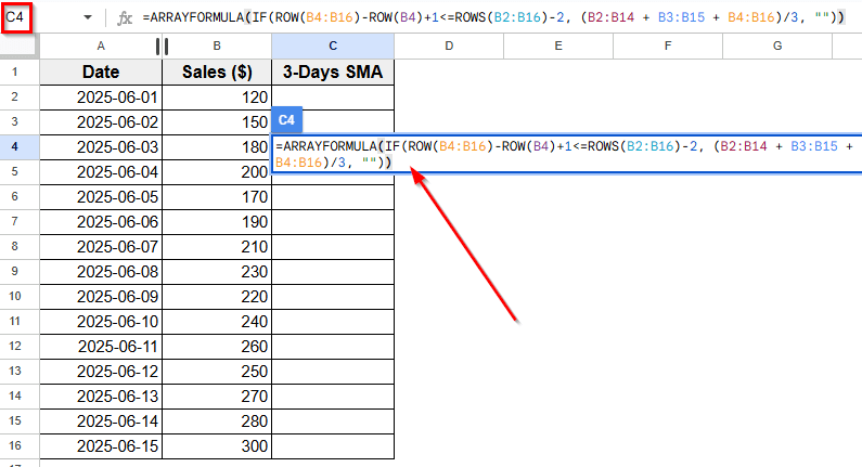
➤ Press Enter.
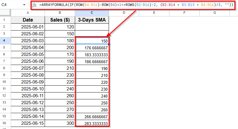
➤ Now Column C will automatically show the 3-day simple moving average, starting from row 4 down to row 16.
Note:
The first two rows remain blank since there isn’t enough data to calculate a full 3-day average.
Combining GOOGLEFINANCE and AVERAGE to Calculate Moving Average
In this method, we’ll take a blank sheet and use GOOGLEFINANCE to pull closing prices for a stock, and then calculate the 3-day simple moving average on that data.
Step 1: Pulling Real-Time Stock Data with GOOGLEFINANCE
Google Sheets has a built-in function called GOOGLEFINANCE that allows you to pull real-time or historical stock data directly into your spreadsheet. This is especially useful when you’re working with stock market trends and want to apply moving averages to track performance over time.
Here is how to apply this method:
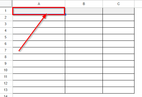
➤ Open your Google Sheets where you want to pull real-time stock data to calculate moving average.
➤ Click on cell A1 in a blank sheet.
➤ Type the following formula to get 15 days of daily closing prices for Google (ticker symbol: GOOG):
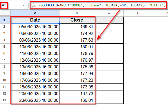
=GOOGLEFINANCE("GOOG", "close", TODAY()-20, TODAY(), "DAILY")
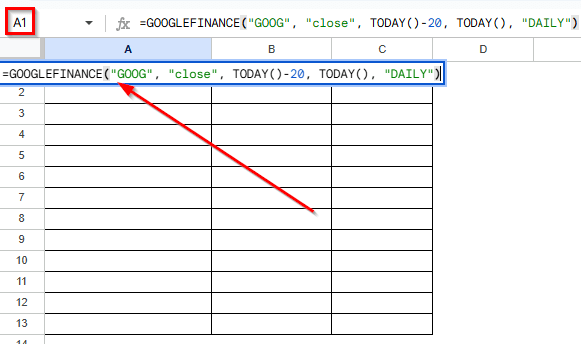
➤ Press Enter.
➤ This will return two columns. Column A shows the dates, and Column B shows the closing prices for each date.
Step 2: Calculating the Moving Average With AVERAGE Function
Once the data is loaded, you can calculate the 3-day moving average just like before.
Here’s how to do that:
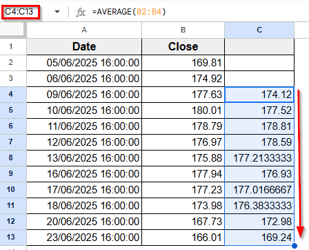
➤ Click on cell C4 from your dataset.
➤ Enter this formula
=AVERAGE(B2:B4)
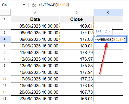
➤ Press Enter. This formula calculates the average of the first three sales values.
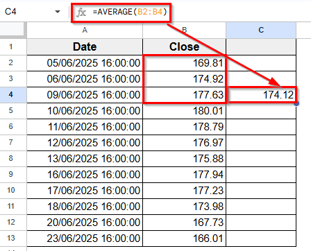
➤ Drag the formula down the column to fill the rest of the moving averages.
Frequently Asked Questions
How do you do a moving average on Google Sheets?
To calculate a moving average in Google Sheets, the most common way is by using the AVERAGE function across a sliding range of rows. Suppose, you want to do a moving average of 7 days.
Here’s how to do that:
➤ Open your Google sheets.
➤ Click on the cell where you want the moving average to appear.
➤ Type the formula to average 7 days of sales, like this: =AVERAGE(B2:B7)
➤ Press Enter. This formula will calculate the 7-day simple moving average across your data.
What is the formula for a moving average?
The most common formula for a moving average is to use the SUM function divided by the number of days. For example, to calculate a 5-day moving average, you can use this formula: =SUM(B2:B6)/5
This adds the values in cells B2 through B6 and divides the total by 5 to get the average.
How to find moving averages in Google Sheets?
To find a moving average in Google Sheets, start by using the GOOGLEFINANCE function to import historical stock prices. Once you have the data, apply the AVERAGE function to calculate a simple moving average over a set number of days.
Wrapping Up
Moving averages help you spot patterns by smoothing out daily changes in your data. In Google Sheets, you can calculate them using different methods depending on your data setup.
Use the AVERAGE function for small ranges, and ARRAYFORMULA function for automatic results across many rows. If you’re tracking stock prices, the GOOGLEFINANCE function lets you pull real-time data and apply moving averages easily.
These functions make it simple to follow trends over time and get clear insights from your spreadsheet.