
In Google Sheets data, we often need to calculate the months between two dates to track the payment cycle, project timelines, or determine an employee’s seniority. To calculate this, we can use the DATEDIF function, and to automate the calculation for required data, we can use the ARRAYFORMULA function. Using the DATEDIF function, we can calculate whole months, partial months, and both months and days.
In this article, I will explain all these methods for accurately calculating the months between two dates in Google Sheets.
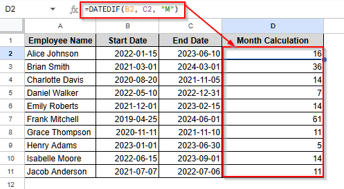
➤ First, select cell D1 and write a suitable name.
➤ Then, click on cell D2 and insert this formula:
=DATEDIF(B2, C2, “M”)
Remember to replace the cell references, B2 and C2, with your data cell references.
➤ Finally, press Enter, and you will see the difference in the whole month. Drag your cursor down to get the months for all of the employees.
Calculate Number of Months Between Two Dates Using DATEDIF Function
If you need to know the difference between two dates in full months, the DATEDIF function is the best choice.
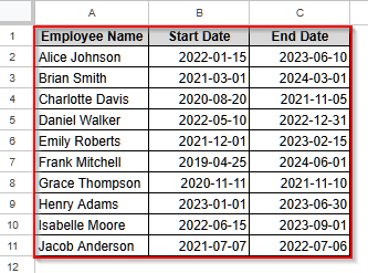
We will use the dataset below to explain how you can use the DATEDIF function to calculate the months between two dates in Google Sheets.
Steps:
➤ First, select cell D1 and write Month Calculation.
➤ Then, select cell D2 and insert the following formula:
=DATEDIF(B2, C2, “M”).
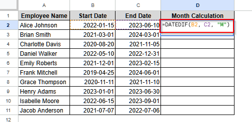
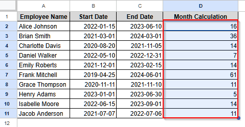
➤ Now, press Enter and drag the cursor to fill in all the employees.
Partial or Fractional Months Calculation Between Two Dates
By modifying the DATEDIF function, we can calculate the partial months between two dates in Google Sheets. It is very useful in case we need to determine the criteria for something like promotion, etc., and need to consider the fractional differences in months, too.
Steps:
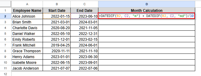
➤ First, select cell D1 and write a name.
➤ Now, click on cell D2 and insert the following formula:
=DATEDIF(B2, C2, “m”) + DATEDIF(B2, C2, “md”)/30.
Remember to replace the cell references, B2 and C2, with your own dataset’s references. Also, here it is assumed that every month has 30 days on average.
➤ Then, press Enter and fill in the formula for all the employees by dragging the cursor of your mouse.
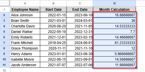
Here, you can see that the month between two dates (start and end date) for employee Alice Johnson is approximately 16.87 months.
Using ARRAYFORMULA Function for Entire Data from Two Columns
When we have a large dataset, manually dragging the cursor to get the calculation for all entries can lead to mistakes. So, we will use the ARRAYFORMULA to make our calculation error-free and save some time.
Steps:
➤ First, select cell D1 and write a name.
➤ Then, click on cell D2 and insert this formula:
=ARRAYFORMULA(DATEDIF(B2:B11, C2:C11, “M”))
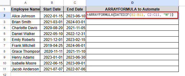
Remember, you can automate most of the calculations with the ARRAYFORMULA function by replacing the cell references with the cell range, like B2 with B2:B11 for our data, as our data is from B2 to B11 cells.
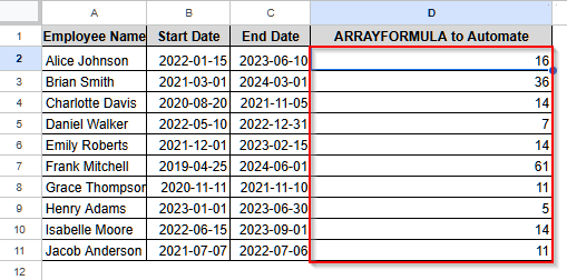
➤ Finally, press Enter, and you will see all calculations returned at once.
Show the Difference Between Two Dates in Both Months and Days
To calculate the months between two dates more accurately, though we can show the fractional months, the fractional value can be confusing. So, to make the calculation visually more appealing and easier to interpret, let’s learn to show the calculation in both months and days.
Steps:
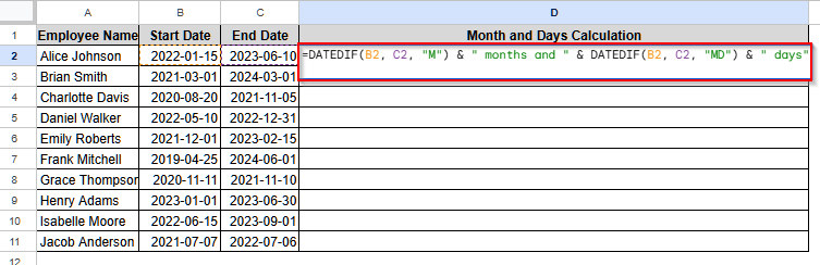
➤ First, select cell D1 and write Month and Days Calculation.
➤ Now, click on cell D2 and insert this formula:
=DATEDIF(B2, C2, “M”) & ” months and ” & DATEDIF(B2, C2, “MD”) & ” days”.
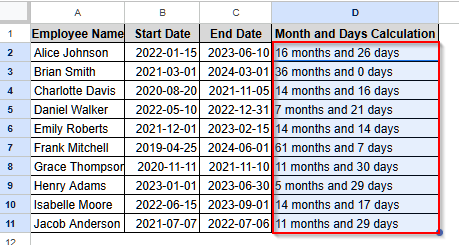
➤ Now, press Enter, and it will return the difference between the two dates in both months and days. Finally, drag the cursor down to fill in all the values.
Frequently Asked Questions
Why Does My DATEDIF Return Date Format instead of Months in Number?
If your cell is formatted as Date instead of Number, you will see the difference between two dates as a date instead of several months. To solve it, first click on the cell with the formula. Then, choose Format from the top menu bar. You will see a list of options open up. Select a Number from that list, and another list will open. Select Number or Automatic, and you will see the months in numbers.
How Can I Count the Months between a Particular Starting Date and Today?
You can simply use the DATEDIF function to calculate the months between a particular starting date and today. Suppose you have a particular date in cell C1. Now, insert this formula in an empty cell: =DATEDIF(C1, TODAY(), “M”). You just need to replace the cell reference C1 with your data reference, and it will return the number of calculated months between that date and today.
How Can I Calculate the Months between Two Dates in the Case of Leap Years?
If you have leap years in your date, you can simply use the DATEDIF function to calculate the months between two dates. This function handles the leap year automatically. In fact, most of the functions in Google Sheets handle leap years automatically. So, you do not need to use any extra method.
Wrapping Up
In this article, we have learned to use the DATEDIF function to calculate months between two dates, both in whole numbers and fractions. Give these methods a try and share your experience with us.