Filtering data effectively is essential when working with large data spreadsheets. Google Sheets simplifies this task with its powerful QUERY function. This feature allows you to search, filter, and manipulate your data using SQL-like commands all within your spreadsheet. It’s specially useful when you need to apply multiple conditions to narrow down your results. Whether you are tracking sales by region, organizing project timelines, or analyzing survey responses, the QUERY function with multiple criteria helps you extract the data you need quickly and effectively.
In this article, we will show you how to use the QUERY function in Google Sheets with multiple criteria. We’ll explore simple ways to filter data based on several conditions, helping you extract the information you need quickly and accurately.
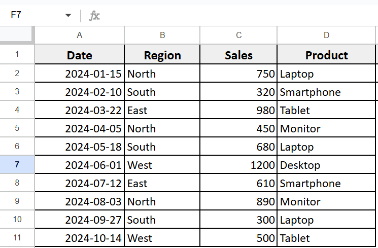
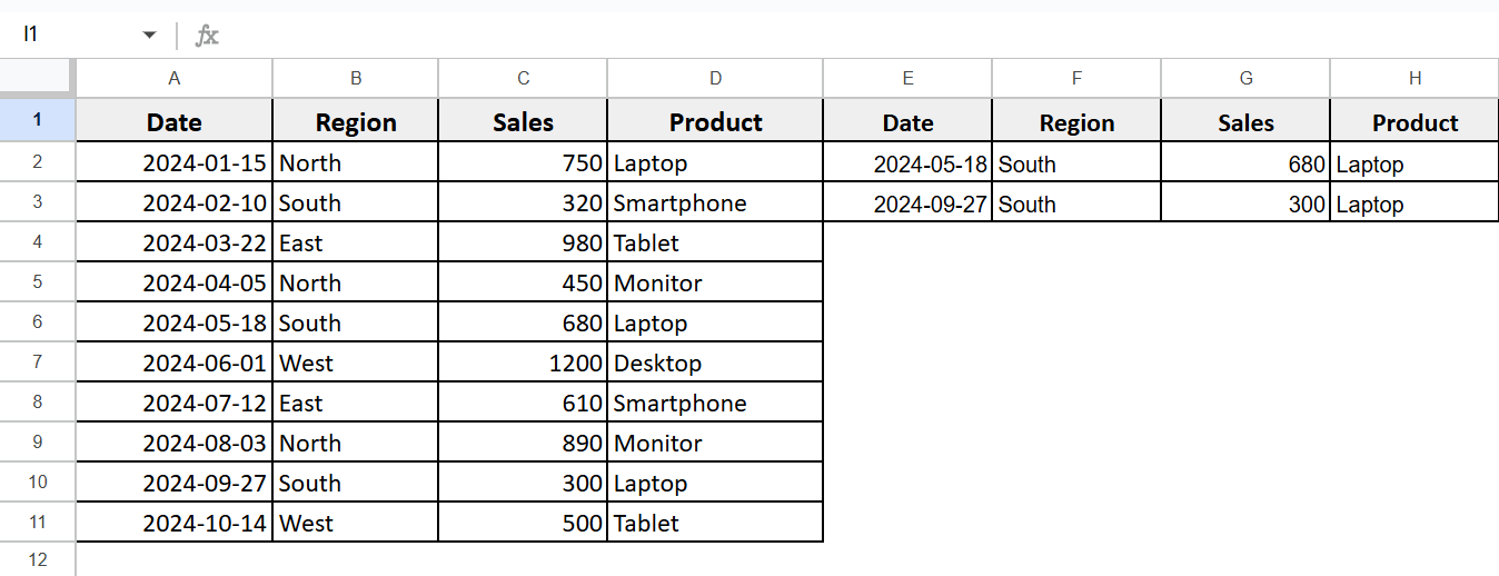
➤ Open your Google Sheet and create a table of four columns (A to D) and name them:
Column A as Date, Column B as Region, Column C as Sales, and Column D as Product.
➤ Leave the Column D empty to apply the function that will return the
➤ Next, apply the QUERY function with the AND condition function in the F2 cell.
➤ Type this formula in cell F2:
=QUERY(A1:D11, “SELECT A, B, C, D WHERE B = ‘South’ AND D = ‘Laptop'”, 1)
➤ Press Enter to implement the formula.
➤ Google Sheets will now return only the rows where Region is South AND Product is Laptop.

Google Sheets Query Using AND Operator
To apply the QUERY function using the AND operator, first you need to set up a structured dataset. Prepare your spreadsheet with columns that contain the data you want to filter, such as dates, names, categories, or values. Then, using the QUERY function, you can combine multiple conditions with the AND operator to return only the rows that match all the specified criteria.
Open your Google Sheet and create a table of four columns (A to D) and name them:
Column A as Date, Column B as Region, Column C as Sales, and Column D as Product.
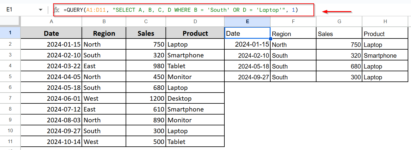
From this dataset, we will extract rows containing both the region as South & the product as Laptop.
Here’s how you can apply this formula:
➤ Apply the QUERY function with the AND condition function in the E1 cell.
➤ Type this formula in cell E1:
=QUERY(A1:D11, “SELECT A, B, C, D WHERE B = ‘South’ AND D = ‘Laptop'”, 1)
➤ Press Enter to implement the formula.
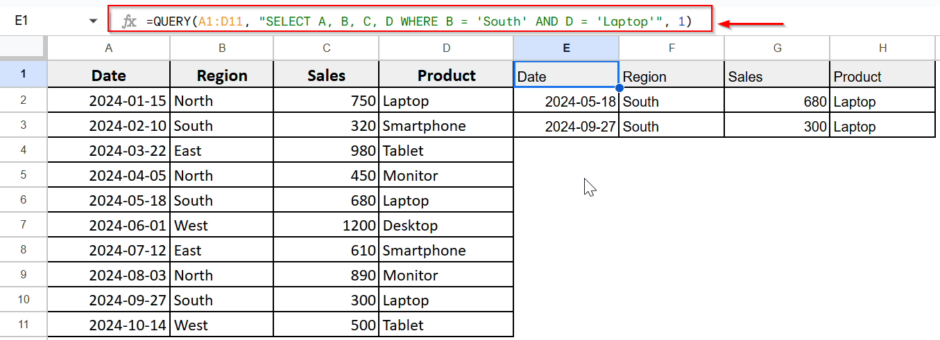
➤ Google Sheets will now return only the rows where Region is South and Product is Laptop.
Google Sheets Query Using OR Operator
While Google Sheets doesn’t have a dedicated button or menu for complex conditions, you can still perform logical operations like OR within your queries by writing them directly into the formula. This lets you retrieve rows that match one condition or another, making it specially useful when working with large datasets where multiple criteria need to be applied flexibly.
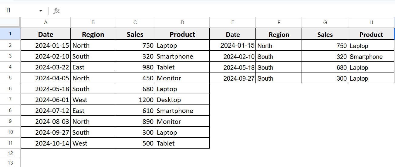
By using OR logic, we will show only the entries from the table where the region is South, or the product type is Laptop.
Steps:
➤ Apply the QUERY function with the OR condition function in the E1 cell.
➤ Type this formula in cell E1:
=QUERY(A1:D11, “SELECT A, B, C, D WHERE B = ‘South’ OR D = ‘Laptop'”, 1)
➤ Press Enter.
➤ It will return rows where the region is South or the product is a laptop.
Combining AND and OR Operators with QUERY
In Google Sheets, the QUERY function lets you use AND and OR to filter data. AND checks if all conditions are true. OR checks if at least one condition is true. You can use both together for more advanced filtering.
This approach is helpful for analyzing data across multiple columns with flexible rules.
From our dataset, we will extract the rows where the region is South & the product is Laptop or the region is North & the product is Monitor.
Steps:
➤ Enter the QUERY formula in the E1 cell.
=QUERY(A1:D11, “SELECT A, B, C, D WHERE (B = ‘South’ AND D = ‘Laptop’) OR (B = ‘North’ AND D = ‘Monitor’)”, 1)
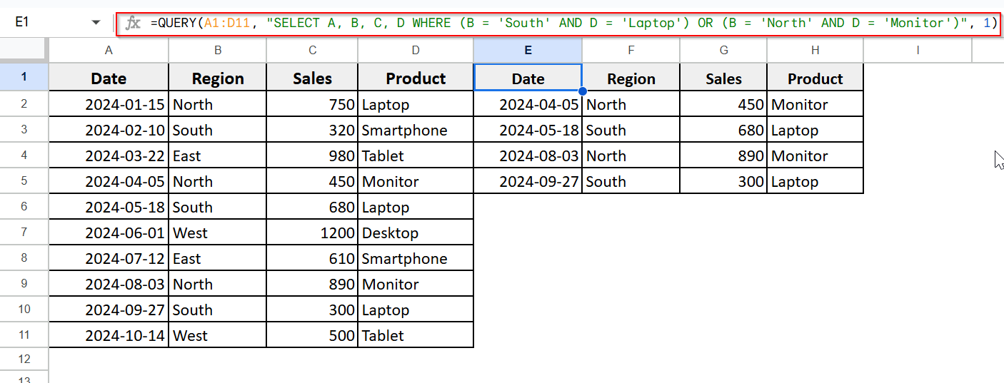
➤ It will return only the rows that match one of these two conditions:
Region is South and Product is Laptop
Region is North and Product is Monitor
Using NOT or Excluding Specific Data
You can exclude specific values or conditions using functions like FILTER, QUERY, or logical operations such as <>. Whether you are excluding products, dates, or regions, NOT logic helps you focus on everything except the values you don’t want and makes your data easier to filter and analyze.
You can continue working with the previous dataset that was created.
Now, suppose you want to exclude all rows where the product is Laptop from your results.
Here’s how you can apply this filter:
➤ Select a blank cell ; E1 and enter the formula
=QUERY(A1:D11, “SELECT A, B, C, D WHERE D != ‘Laptop'”, 1)
To exclude all rows with the product Laptop.
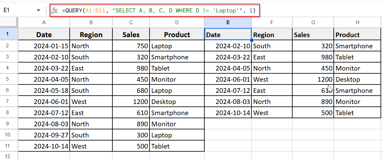
➤ Now you will see all rows except those where the product is a laptop.
Frequently Asked Questions
Can I exclude multiple values?
Yes, use multiple conditions with the (AND) operator:
=FILTER(A2:B10, (B2:B10 <> “Laptop”) * (B2:B10 <> “Tablet”))
What if I want to exclude blank cells?
Use this in QUERY: =QUERY(A1:D10, “select * where D is not null”, 1)
How do I exclude a value using the FILTER function?
Use the <> operator.
Wrapping Up
In this article, we explored how to use the QUERY function in Google Sheets with multiple criteria. We’ve seen how this flexible method can help you filter complex datasets more precisely and make your data analysis more efficient and targeted.