Google Sheets FILTER with the OR Condition (3 Useful Examples)

We use the FILTER with OR condition in Google Sheets when we want to include values that meet any one of a preset list of multiple criteria. For example, if you have customers of various ages from different countries, and you want to list customers from Canada or the USA.

In this article, we will explain how to modify the FILTER function to use the OR condition in a sample Google Sheets dataset.

Key Takeaways

➤ First, select cell E1 and give it a name.
➤ Then, select cell E2 and insert this formula.
=FILTER(A2:D15, (C2:C15=”Canada”) + (C2:C15=”USA”)).
➤ Finally, press Enter to get the filtered data for country Canada or the USA.

Download Practice Workbook

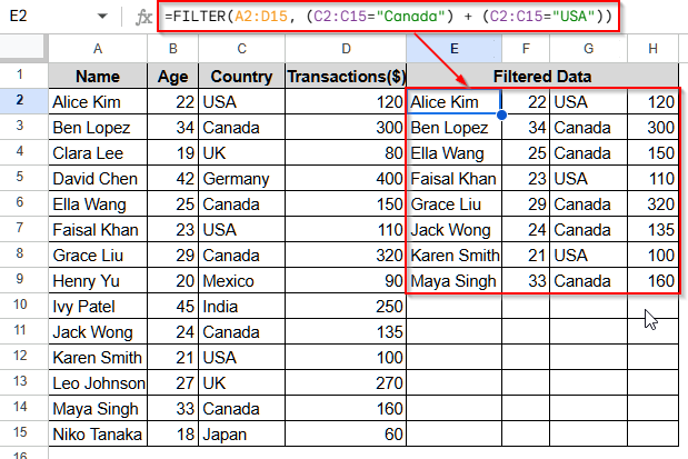
Using FILTER Function Applying OR Condition in Google Sheets

The FILTER function in Google Sheets is a powerful data analysis tool that can be easily adjusted to accommodate various conditions, such as the OR condition.

We will use the dataset below to explain how you can use the FILTER function with OR condition in Google Sheets.

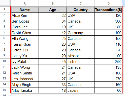
This is a global customer dataset of a company that includes customers’ names, age, country, and transactions they made on that day. We need to find the list of customers who are from the country Canada or the USA.

Steps:

➤ First, select cell E1 and write Filtered Data.
➤ Then, click on cell E2 and insert the following formula:

=FILTER(A2:D15, (C2:C15=”Canada”) + (C2:C15=”USA”)).

Explanation

In this formula, the “+” sign works as the OR condition. It tells the Filter function to return the values for Canada or the USA.

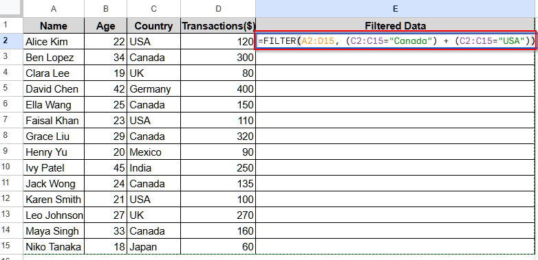
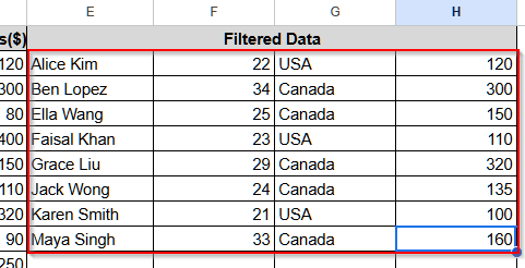
➤ Finally, press Enter, and you will see the filtered dataset for country Canada or the USA.

Explanation

Here, the filtered dataset is returned in columns E to H. Also, the columns correspond to the original dataset, that is, column E is Name, column F is Age, column G is Country, and column H is Transaction ($). Also, in column G (the filtered Country), there are only countries Canada or the USA; other countries are filtered out.

FILTER With OR Condition for Multiple Column Criteria

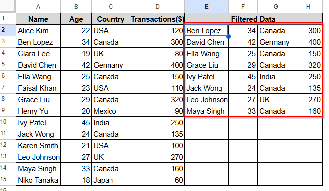
The OR condition can be applied to filter out data for criteria on multiple columns. For example, if we want to see the customers who live in Canada or who have made transactions over $150, we can use the Filter function with OR condition. For this purpose, we will use the previous dataset.

Steps:

➤ First, select cell E1 and give it a name.
➤ Now, click on cell E2 and insert this formula:

=FILTER(A2:D15, (C2:C15=”Canada”) + (D2:D15>150))

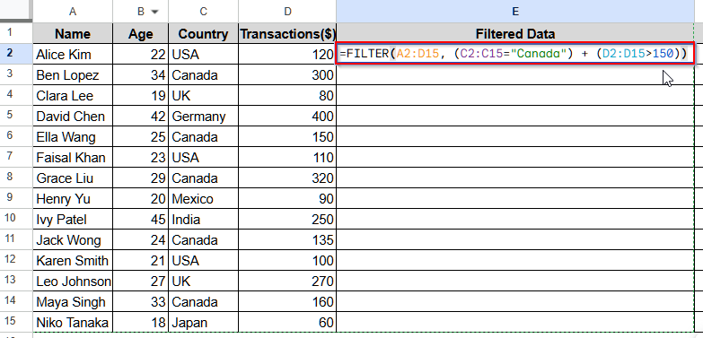
➤ Then, press Enter, and it will return the filtered dataset with entries only for Canada or Transaction ($) more than $150.

FILTER Function with More Than Two OR Conditions in Google Sheets

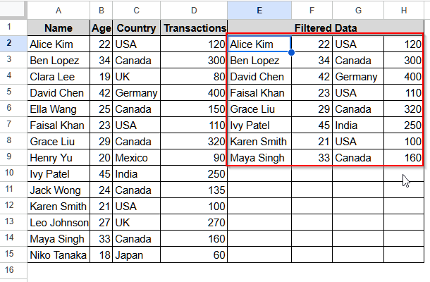
To use the Filter function with more than two OR conditions in Google Sheets, we can simply add those conditions using the “+” sign. Let’s take a look at the demonstration below using the same dataset. We will filter the dataset for customers with an age of more than 30 years, or customers who live in the USA, or customers who made Transactions ($) over 300.

Steps:

➤ First, select cell E1 and name it.
➤ Now, click on cell E2 and insert this formula.

=FILTER(A2:D15, (B2:B15>30) + (C2:C15=”USA”) + (D2:D15>300))

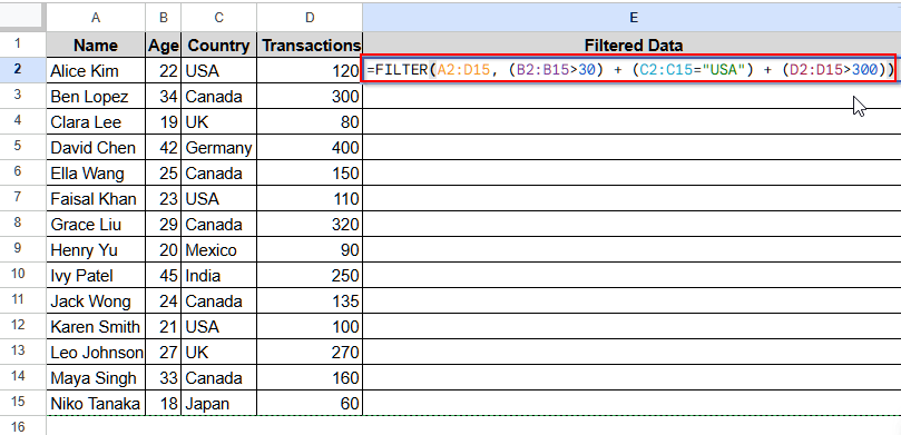
➤ Press Enter, and you will see the filtered data.

Frequently Asked Questions

Can I Directly Use the OR Function Inside FILTER Function in Google Sheets?

No, you cannot use the OR condition directly inside the Filter function as a nested function in Google Sheets. Instead, you need to use the “+” sign. It adds a clause and works as the OR condition.

Can I Use “,” (Comma) Instead of “+” Sign to Add OR Condition with Filter Function?

No. Because conditions separated by “,” (comma) with the Filter function represent AND logic. That is, all the conditions separated by a comma must be true to return a value. So, you cannot use “,” instead of the “+” sign to apply OR logic or condition with Filter function in Google Sheets.

Can I Use FILTER with OR Condition on Data from Different Sheets?

Yes, you can filter data from a different sheet to a new sheet using the Filter function with OR condition. Let’s say our dataset is in Sheet1 and we want to see the filtered data in another sheet. Then, you need to use the following formula:
=FILTER(Sheet1!A2:D15, (Sheet1!C2:C15=”Canada”) + (Sheet1!C2:C17=”USA”)).

Wrapping Up

In this article, we learned how to use the FILTER function in Google Sheets with the OR condition. Inside the FILTER function, this condition is represented by the plus sign (“+”). And, you can easily add two or more conditions using this sign to apply the OR logic. Give it a try and share your experience with us.

Post Views: 7