In Excel, it is important to know how to transfer data from one worksheet to another using Vlookup, especially if you are working with multiple worksheets. While VLOOKUP function is the go-to method for transferring data across worksheets, there are also alternative methods that allow users to perform this task efficiently.
Follow the steps below to transfer data from one Excel worksheet to another automatically using the VLOOKUP function.
➤ In your dataset, select the cell where you want to display the transferred data and put the following formula:
=VLOOKUP(lookup_value, table_array, col_index_num, [range_lookup])
➤ Replace lookup_value with the value that you want to find in the first column of your lookup table.
➤ Replace table_array with the range of cells that contains the data you are searching for.
➤ Replace col_index_num with the column number in the table array, from which to return the value.
➤ Replace [range_lookup] with FALSE to display an exact match or TRUE for a partial match.
In this article, we will learn two effective methods of transferring data from one Excel worksheet to another using VLOOKUP. Additionally, we will also explore two powerful alternatives to the VLOOKUP function for transferring data across worksheets more efficiently.
Use VLOOKUP Function to Transfer Data from Another Worksheet
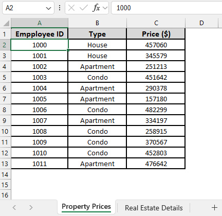
In the sample dataset, we have two worksheets, one called “Property Prices” containing information about Employee ID, Property Type and Property Price. And the other called “Real Estate Details” where we have Employee ID, Listed By, City and an empty Price column.
![]()
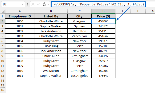
Using the VLOOKUP function, we will transfer the corresponding property price from the “Property Prices” worksheet into column D of the “Real Estate Details” worksheet, based on matching Employee ID values. We will display the updated dataset in a separate worksheet called “VLOOKUP Function”.
VLOOKUP in Excel is an important function which allows users to search for a specific value in the first column of a range or table and return a corresponding value from another column in the same row.
Steps:
➤ Open the VLOOKUP Function worksheet and in cell D2, put the following formula:
=VLOOKUP(A2, ‘Property Prices’!A2:C13, 3, FALSE)
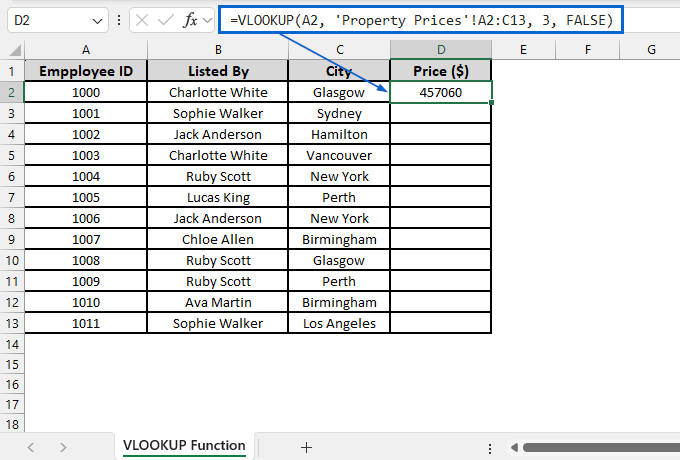
➧ “A2” is the lookup value that we are searching for in the first column of the range.
➧ “Property Prices'!A2:C13” part specifies the lookup range in the Property Prices worksheet where Employee ID and Price are stored.
➧ “3” is the column index number in the lookup range from which to return the price value.
➧ “FALSE” tells the formula to return an exact match.
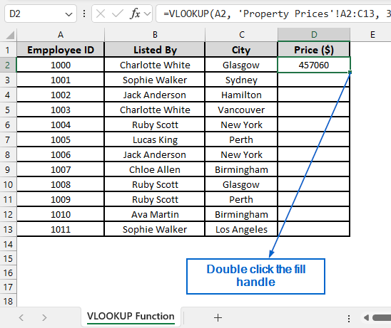
➤ Next, double-click the fill handle located in the bottom right corner of cell D2 to apply the formula across the entire column.
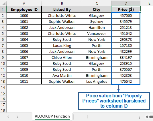
➤ The corresponding price values from the Property Prices worksheet should now be visible in column D.
Use VLOOKUP with Named Range
A named range in Excel is a user-defined descriptive label assigned to a specific cell or a range of cells. Instead of using a direct cell reference like in the previous method, we will define a named range for this dataset and transfer price data from Property Price worksheet to column D of the Real Estate Details worksheet. We will display the updated dataset in a separate VLOOKUP with Named Range worksheet.
Steps:
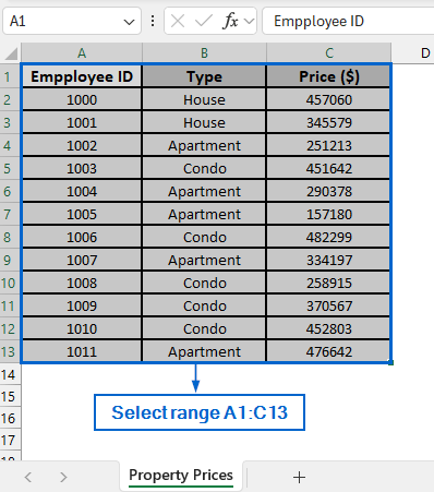
➤ Open the Property Price worksheet and select the range A1:C13.
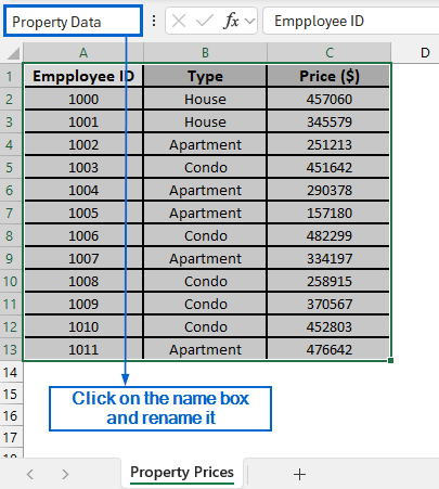
➤ Click on the Name Box located at the top-left corner and rename it to PropertyData.
➤ Next, head to VLOOKUP with Named Range worksheet and in cell D2, put the formula:
=VLOOKUP(A2, PropertyData, 3, FALSE)
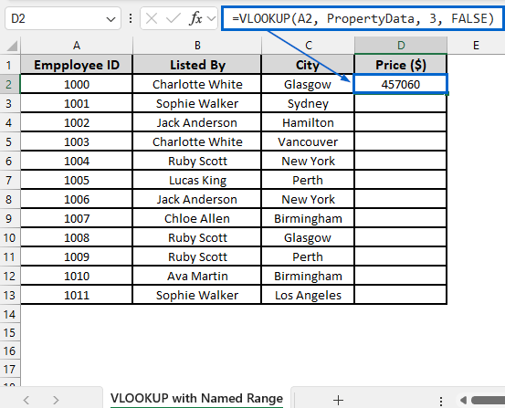
➧ PropertyData is the named range that replaces the direct reference 'Property Prices'!A2:C13 used in the previous method. It makes the formula easy to read and manage.
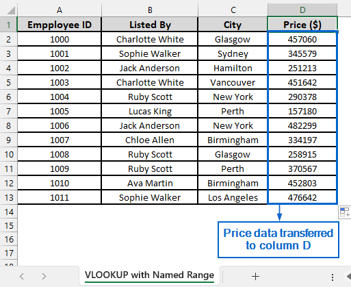
➤ Then, double click on the fill handle and apply the formula across column D.
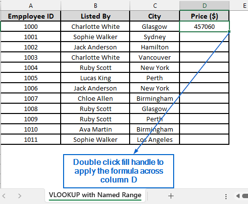
➤ Column D should now display the transferred price data.
Alternatives to the VLOOKUP Function for Data Transfer Across Worksheets
While the VLOOKUP function is widely used for transferring data across multiple worksheets, it has some major drawbacks. One key limitation of the VLOOKUP function is that it can only search for a value in the first column of the lookup range and return data from columns to the right, restricting flexibility. In contrast, the XLOOKUP function provides more flexibility by allowing for searches in any column irrespective of direction.
Similarly, INDEX with MATCH provides even more versatility, supporting lookups in any columns, handling multiple criteria and offering better performance in large datasets
Use XLOOKUP Function for a More Flexible Approach
This is another effective method that utilizes the XLOOKUP function to transfer data from one worksheet to another in Excel automatically. Unlike the VLOOKUP function, XLOOKUP can search for values in any column, meaning the lookup key does not need to be in the first column of the data range.
We will again work with the same dataset and transfer price data from the Property Prices worksheet to column D of the Real Estate Details worksheet. The updated dataset will be stored in a separate worksheet called XLOOKUP Function.
Steps:
➤ Open the XLOOKUP Function worksheet and in cell D2, put the following formula:
=XLOOKUP(A2, ‘Property Prices’!A2:A13, ‘Property Prices’!C2:C13)
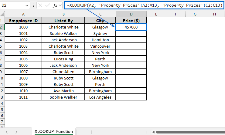
➧ “A2” indicates the lookup value that we want to find.
➧ “'Property Prices'!A2:A13” indicates the range of columns where Excel searches for the lookup value in the Property Prices worksheet.
➧ “'Property Prices'!C2:C13” is the column from which Excel returns the result into our worksheet.
➤ Then, select cell D2 and double click on the fill handle to apply the formula across column D.
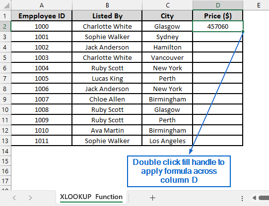
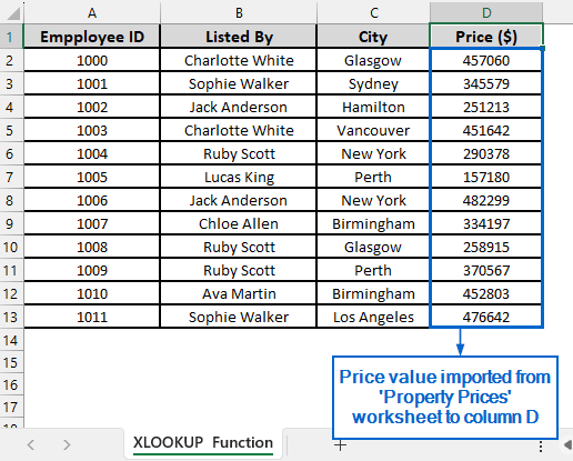
➤ Column D should now display the price values transferred from the Property Prices worksheet.
Use INDEX-MATCH Formula for Advanced Lookup
This is an advanced method that can handle complex lookups with multiple criteria by using the INDEX and MATCH functions. The INDEX and MATCH functions in Excel are used together to retrieve values from a dataset by locating the position of a specific value (MATCH) and returning the corresponding value from a specified row or column (INDEX).
We will again work with the same dataset to transfer the price information from the Property Prices worksheet into column D of the Real Estate Details worksheet. The modified dataset will be stored in a separate “INDEX and MATCH Function” worksheet.
Steps:
➤ Open the INDEX and MATCH Function worksheet and in cell D2, put the following formula:
=INDEX(‘Property Prices’!C2:C13, MATCH(A2, ‘Property Prices’!A2:A13, 0))
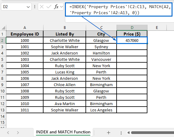
➧ MATCH(A2, 'Property Prices'!A2:A13, 0) searches for the exact value in cell A2 within range A2:A13 of the Property Prices worksheet.
➧ INDEX('Property Prices'!C2:C13, …) takes the position number provided by MATCH and returns the value from the same row in the C2:C13 range of the Property Prices worksheet.
➤ Then, apply the formula to the remaining cells by double-clicking the fill handle of cell D2.
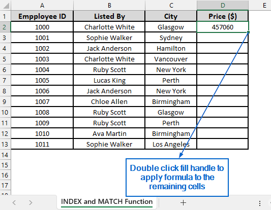
➤ Transferred price values from the Property Prices worksheet should now be displayed in column D.
![]()
Frequently Asked Questions
Will My Dataset Update Automatically If Any Changes Are Made to the Source Worksheet?
Yes, when you use functions like VLOOKUP, XLOOKUP, and INDEX with MATCH to transfer data, the output will update automatically when you make any changes to the source worksheet. Just make sure that cell references and worksheet names remain the same.
Which Method is Best for Beginners When Transferring Data Between Worksheets?
If you are a beginner and want to transfer data between different worksheets, the VLOOKUP function method would be the best one for you. It has simple syntax and is easy to use, making it ideal for basic lookup tasks.
Concluding Words
Knowing how to transfer data automatically between Excel worksheets is a valuable skill that helps users streamline datasets and enhance data organization. In this article, we have explored three efficient methods of transferring data from one Excel worksheet to another, including using the VLOOKUP Function, XLOOKUP Function and combining INDEX with MATCH Function. Make sure to try each method and select one that best aligns with your needs.