In Excel, we often need to work with large datasets. And, finding specific data from them is not an easy task. However, users often must extract multiple values based on specific conditions or criteria. For instance, users might need to pull out the order placed by a specific customer, or the names of the employees working under one department. In this situation, most of your resultant value is not singular; you need to look for multiple values here. Unlike single values, multiple ones can’t be returned with a straightforward function or lookup. As a result, users often need to modify the formula to get the desired output.
Follow the steps below to find multiple values in Excel based on specific criteria.
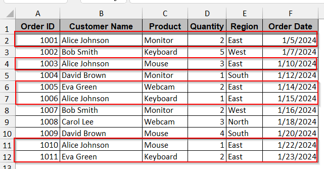
➤ Select the entire dataset and go to the Data tab.
➤ From the ribbon, choose the Advanced option under Sort and Filter.
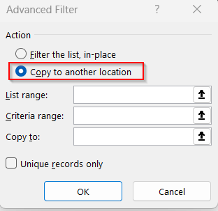
➤ The Advanced Filter window appears. Under Action, check Copy to another location to paste the new table in a separate cell.
➤ In the Criteria range, select the column and the cell with the condition you want to match.
➤ Select a new cell in the Copy to option where your filtered table will be visible.
➤ Click OK to filter the list based on one criterion.
In this article, you will move into the nitty-gritty of the methods that can help you find multiple values in Excel. With the single functions and options like FILTER and Advanced Filter, a combination of formulas of TEXTJOIN and INDEX-SMALL-IF, and even automated tools like Power Query and VBA macros, you can easily extract more than one value under one condition. So, stay tight as you guide yourself through each with detailed steps and interactive examples.
Excel’s Dynamic FILTER Function for Multiple Value Criteria
The FILTER function is the most basic and easiest to pull out multiple values under one criterion or condition. It returns not only the rows for the existing values but also the columns. Without manual filtering and complex VBA codes, it is the best of both worlds.
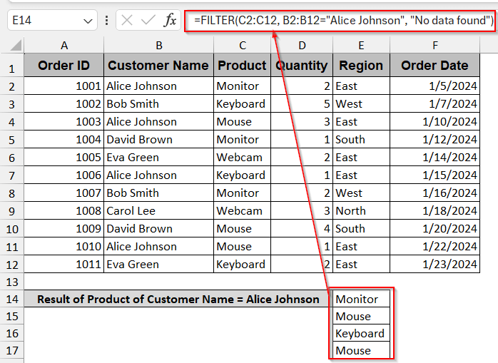
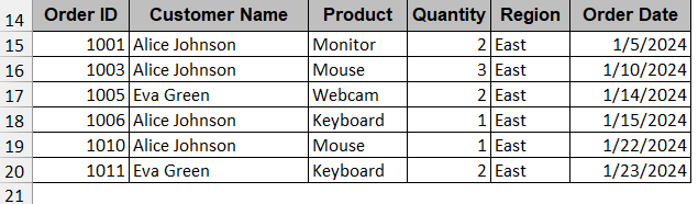
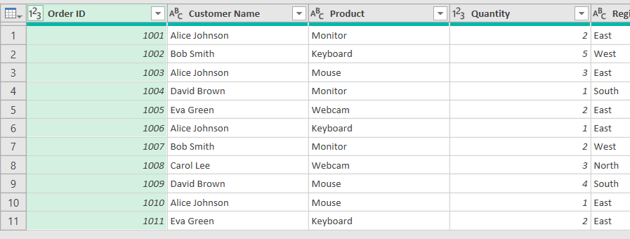
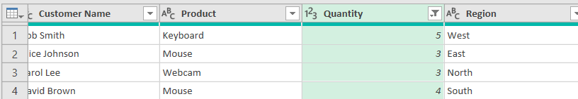
In this example, we will be dealing with the datasheet of the customer’s order details, location, and quantity. With this FILTER function, we want to extract all the values or, more specifically, product names purchased by a single customer. Here, our chosen condition is the ‘Alice Johnson’ from the column Customer Name.
Steps:
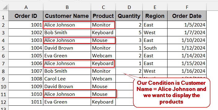
➤ Select an empty cell where you want the filtered data to appear and give it an appropriate header.
![]()
➤ Enter the formula for the FILTER function –
=FILTER(array, include, [if_empty])
➤ Replace the array part with the range of the table (e.g., A2:F12).
➤ In the include part, write the cell number and column along with the condition (e.g., B2:B12= “Alice Johnson”)
➤ If the condition is not met, the function is false. It shows #CALC!error. Replace the [if_empty] part with “No orders found” or any string that will be displayed if no data is found with the condition stated.
➤ Press Enter to display the filtered datasets.
Note:
➨ You can also include multiple conditions using this FILTER function –
=FILTER(A2:F12, (B2:B12=”Alice Johnson”)*(E2:E12=”East”), “No matching orders”)
Here, the conditions filter the data having the customer name ‘Alice Johnson’ and the region ‘East’.
➨ The FILTER function is only applicable in Microsoft 365 and 2021. Versions older than this and the Excel web version are not programmed with this function.
List Multiple Matches using TEXTJOIN and FILTER
Though FILTER is an efficient way to share all the values that fulfill the conditions, sometimes it is not enough. If you want to display all the matching cells in a single cell, separated by some delimiter like a comma or a semicolon, then using the TEXTJOIN will be a better approach. To achieve this flexibility, you must combine the TEXTJOIN function with an extra FILTER function.
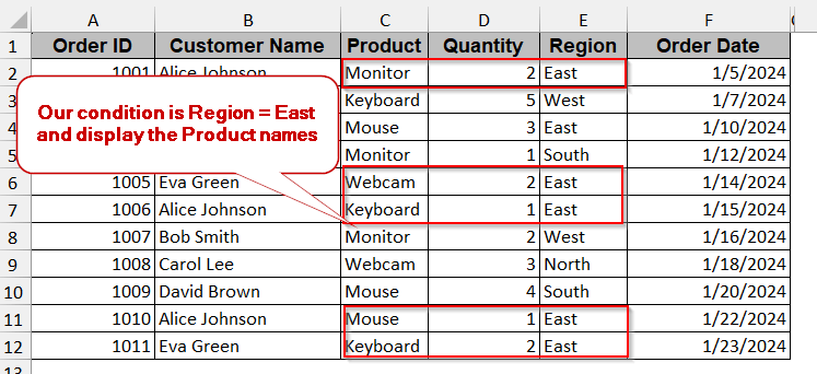
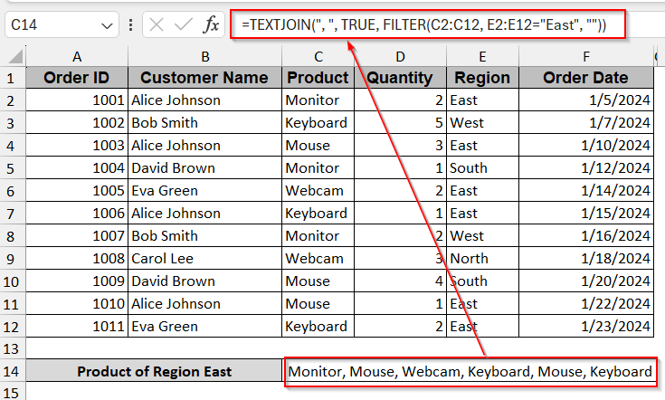
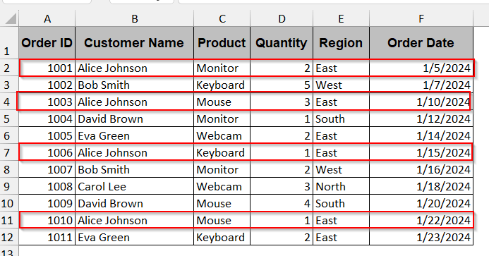
The same example of the dataset will also be discussed here. However, here we will be displaying the cells having the Region as ‘East’ from column E.
Steps:
➤ Select a cell where you want the concatenated list to be displayed with a header if required.
![]()
➤ Enter the TEXTJOIN function combined with the previous FILTER function.
=TEXTJOIN(", ", TRUE, FILTER(array, include, ""))
Here, the “,” is the delimiter; that means a comma will separate the values. The value TRUE is used to ignore any empty cells that are generated from the inner FILTER function when the condition is not met.
➤ Replace the array with the column range you want to display for the specific condition (e.g, C2:C12).
➤ In the include portion, write the condition and the column and cell number (e.g., E2:E12= “East”).
➤ Press Enter to view the filtered value of the products having the Region in ‘East’ in column E.
Note:
➨ Only supported in Microsoft 365 and 2021. Older versions do not have the FILTER function.
➨ You can set the delimiter to the next line instead of a comma or semicolon using the CHAR(10) in the TEXTJOIN function.
INDEX-SMALL-IF Formula for Array-Based Multiple Match
As the FILTER and TEXTJOIN methods are specifically curated for users with the newer Excel versions, we need a dynamic approach for older versions. The combination of INDEX, SMALL, and IF is your go-to method if you do not have the latest Excel versions. It is like an array-based formula that works similarly to the FILTER function for the legacy versions.
With the same example, we will filter the Order ID with the Product = ‘Mouse’ from column C.
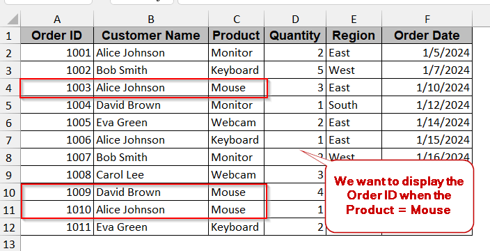
Steps:
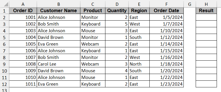
➤ Create a separate column to display the results as they are generated in vertical form.
➤ In the selected cell, write the following formula –
=IFERROR(INDEX([Return_Column_Range],SMALL(IF([Criteria_Column_Range]=[Your_Criteria_Value],ROW([Criteria_Column_Range])-MIN(ROW([Criteria_Column_Range]))+1),ROWS([First_Result_Cell]:[Current_Result_Cell]))),"")
➤ Replace the [Return_Column_Range] with the column range that you want to display as results. (e.g, A2:A12).
➤ Inside the SMALL function, replace the [Criteria_Column_Range]=[Your_Criteria_Value] with the column range containing the condition and the condition (e.g, $C$2:$C$12=”Mouse”)
➤ In the next part of the function ROW([Criteria_Column_Range])-MIN(ROW([Criteria_Column_Range]))+1), enter the column range of the condition and the add one with the first cell number of the data to ensure the values match the row sequence (e.g- ROW($C$2:$C$12)-ROW($C$2)+1)).
➤ Inside the last ROW function, write the cell range where you want to display the values (e.g, ROWS(H$2:H2)).
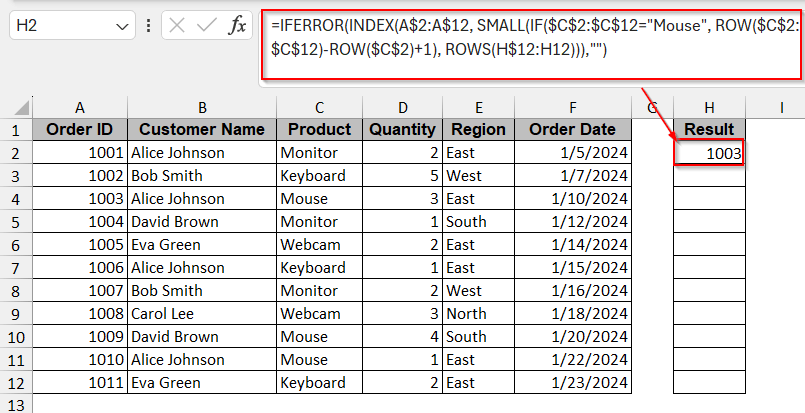
➤ The entire formula will look like this –
=IFERROR(INDEX(A$2:A$12, SMALL(IF($C$2:$C$12="Mouse", ROW($C$2:$C$12)-ROW($C$2)+1), ROWS(H$12:H12))),"")
➤ Press Ctrl + Shift + Enter simultaneously. It tells Excel that the formula is array-based.
➤ Drag the cells or use Fill Handle to apply the same formula to the rest of the cells.
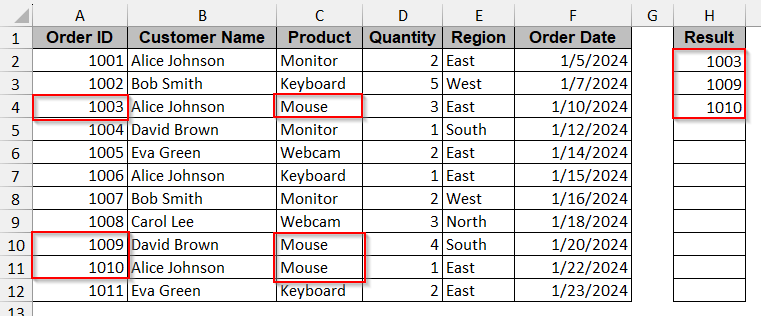
It will only display the Order ID with the mouse product.
Note:
➨ Make sure to press Ctrl + Shift + Enter to generate the value.
➨ The INDEX-SMALL IF function is not dynamic. If any cells are updated or deleted, you need to rewrite the formula again to display the updated results.
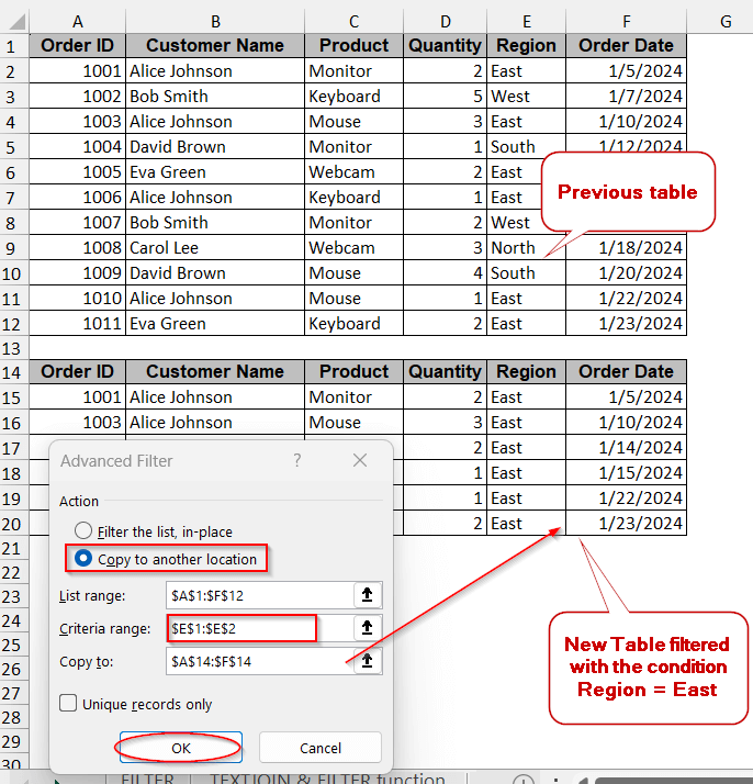
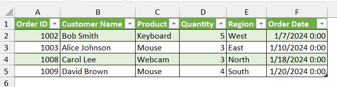
Advanced Filter Option Using One Condition
Advanced Filter can be used in any version of Excel. Instead of complex formulas, you can generate a separate table or filter the existing table with the same condition.
To understand this method, we will filter all the rows with the Region value of ‘East’.
Steps:
➤ Select the entire dataset and go to the Data tab.
➤ Click on the Advanced option under the Sort & Filter option to open the Advanced Filter option.
➤ Under Action, select Copy to another location to generate a new filtered table.
➤ Ensure the List range is set to the entire dataset.
➤ Select the Criteria range as the condition along with the cell and the column range (e.g, E2:E12= “East”)
➤ In the Copy to, select the cell number from which you want to spill the data.
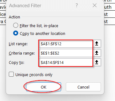
➤ Click OK to generate the new list. The new table will show only the rows with ‘East’ as the Region value.
Note:
You can also modify and filter the data in the same table. Just check Filter the list, in place instead of Copy to another location. However, the previous data can’t be retrieved and will be lost forever.
Search Multiple Values Dynamically Using VBA Macros
All the previous methods are good enough to extract multiple values from smaller datasets. When you need to deal with larger datasets, with thousands of redundant data points, your problem needs an automated solution. And what else can it be rather than VBA? You can modify and customize your VBA code to make the search interactive.
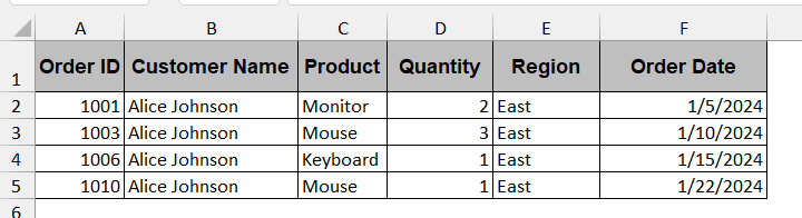
Here, we will retrieve all the orders placed by a specific customer (e.g – ‘Alice Johnson’) with an input box. The filtered data will be generated in a different worksheet.
Steps:
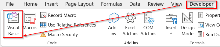
➤ Go to the Developers tab -> Visual Basic to launch the VBA editor.
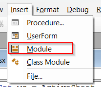
➤ In the VBA editor, click the Insert menu -> Module.
➤ Paste the following code in the blank space below –
Sub GetRowsByCustomerName()
    Dim ws As Worksheet, outputWs As Worksheet
    Dim lastRow As Long, outputRow As Long
    Dim searchName As String
    Dim i As Long
    Set ws = ActiveSheet
    searchName = InputBox("Enter the Customer Name:")
    If searchName = "" Then Exit Sub
    Set outputWs = Worksheets. Add
    outputWs.Name = "Results_" & Replace(searchName, " ", "_")
    ws.Rows(1).Copy Destination:=outputWs.Rows(1) ' Copy headers
    lastRow = ws.Cells(ws.Rows.Count, 2).End(xlUp).Row ' Column B = Customer Name
    outputRow = 2
    For i = 2 To lastRow
        If Trim(ws.Cells(i, 2).Value) = Trim(searchName) Then
            ws.Rows(i).Copy Destination:=outputWs.Rows(outputRow)
            outputRow = outputRow + 1
        End If
    Next i
    If outputRow = 2 Then
        MsgBox "No matching records found for: " & searchName
        Application.DisplayAlerts = False
        outputWs.Delete
        Application.DisplayAlerts = True
    End If
End Sub
➤ Save the VBA code and close the window.
➤ Click on Macros beside the Visual Basic option.
➤ In the Macros window, select the function name.
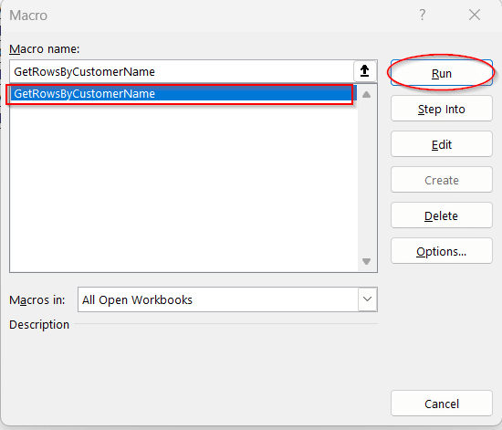
➤ Clicking on Run will generate a new worksheet containing the product details or the rows with the customer’s name, ‘Alice Johnson’.
Note:
When no matching data is found, the new worksheet is automatically deleted.
Apply Conditional Filtering with Power Query to Find Multiple Values
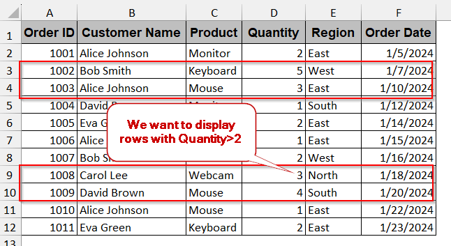
For advanced searching and filtering, the most preferred option is Power Query. It not only pulls multiple data from a single condition, but it also enables you to set extra conditions rather than simple values. In this method, we will try to retrieve the data of the products from the previous datasheet, having a quantity greater than 2.
Steps:
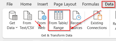
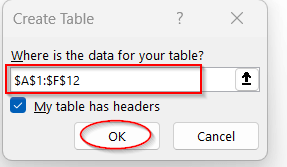
➤ Select the entire dataset and go to the Data tab.
➤ From the Data tab, select From Table/Ranges.
➤ A dialog box appears, ensuring the selected table range. Check the box My table has headers option for the proper table loading.
➤ A Power Query window will be launched, displaying the entire dataset.
➤ Select the column in which you have the conditions. For example, to set the quantity greater than 2, select the column Quantity.
➤ In the header, click on the arrow or menu sign.
➤ In the drop-down menu, select the Number Filter option. Select the type of condition you want to specify. We will be choosing Greater than as per our requirement of the example.
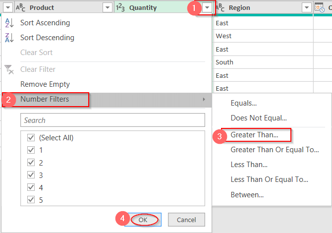
➤ In the Filter Row window, select the value of greater than (e.g, 2)
➤ If you want to specify more conditions, you can select And and add more.
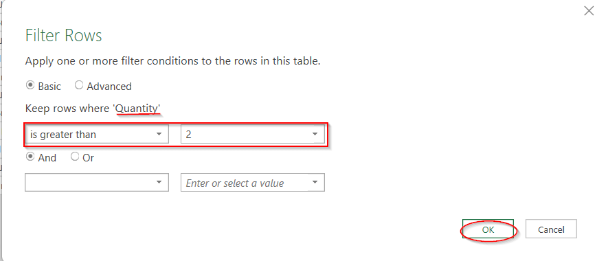
➤ When done, click OK.
➤ This will reduce the table in the editor and display only the rows with a Quantity value greater than 2.
➤ Click on the Close and Load option in the Home tab.
➤ This will create a new worksheet with the rows that satisfy your conditions.
Note:
You can also give two or more conditions and display rows if only one condition is satisfied. For example, the rows having the Quantity value greater than 2 and the Order Date less than 1/20/2024. You need to select the OR option and add more conditions in the Filter Row window.
Frequently Asked Questions
Can Excel return multiple values for one lookup?
The previous lookup functions, like VLOOKUP and HLOOKUP, cannot return multiple values for one condition. However, the modern versions use XLOOKUP, which can return multiple values when searched.
What function returns multiple matching values?
Microsoft 365 and 2021 have functions like FILTER and TEXTJOIN to search for multiple values in Excel. For versions older than, you can use INDEX-SMALL IF to get the job done.
Can I use VLOOKUP to return multiple values?
VLOOKUP can only return one value corresponding to the first match it found based on the condition. To use the regular VLOOKUP, you need to add extra functions to return multiple values.
Why is FILTER not working to return multiple values?
The FILTER function does not work in Excel versions older than 2021. To use the function, you need Microsoft 365 or 2021.
How can I get multiple values from a drop-down list in Excel?
The general Excel drop-down list only enables single-value selection. To get the multiple values from the drop–down list, you can customize your VBA code snippet. With the help of the Macros, you can get this selective functionality.
Concluding Words
Finding multiple values in Excel can be complicated until you know the best methods. With the one-click functions like FILTER and TEXTJOIN, you can easily extract multiple rows that have the same conditions. For older versions, INDEX-SMALL IF can be a better function. Again, there are options like Advanced Filter, powerful VBA Macros, and Power Query to simplify the task with some tweaks.
Don’t be overwhelmed by seeing all these methods. Go through them one by one and download our worksheets to find the right pick for you.