Merging duplicate rows is a common data-cleaning task in Excel, especially when you’re working with sales data, customer lists, or reports that contain repeated entries. While Excel doesn’t have a direct “merge duplicates” button, it does provide several powerful features that can help you consolidate, clean, and restructure your data efficiently. Whether your goal is to sum values, combine text, or simply remove redundant entries, there are multiple techniques suited for different types of data and use cases.
While Excel doesn’t offer a one-click “merge duplicates” option, In this article, we’ll walk through several effective methods to merge duplicate rows in Excel starting from simple formulas and built-in tools like Consolidate, to more advanced solutions like PivotTables, Power Query, and VBA macros. Let’s get started.
Steps to merge duplicate rows in Excel:
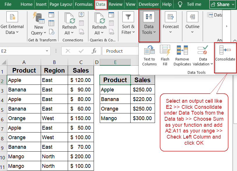
➤ Select a blank cell where you want to display the summarized results (e.g., E2).
➤ Go to the Data tab and click Consolidate under Data Tools.
➤ In the Function dropdown, select Sum to total the sales.
➤ In the Reference box, select your full dataset (A1:C11) and click Add.
➤ Check both Top row and Left column or either of them to let Excel use your headers for grouping.
➤ Click OK.
Use the Consolidate Tool to Summarize Duplicate Rows
If you want to merge duplicate entries by summing their values such as calculating the total sales per product, Excel’s built-in Consolidate feature is a quick and effective solution. It automatically groups rows with the same labels and performs a calculation, such as Sum, on the corresponding values. This method works best when you’re focused on summarizing one column of numeric data, like Sales, based on a single category such as Product.
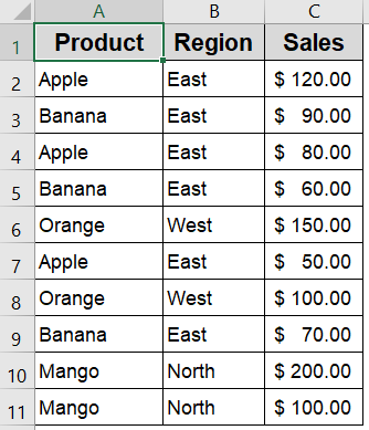
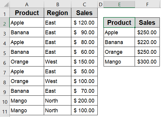
We’ll use a sample dataset that lists sales figures by Product and Region, with some entries appearing multiple times with different sales values.
Steps:
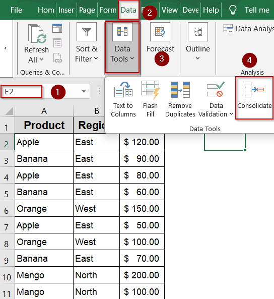
➤ Select a blank cell where you want to display the summarized results (e.g., E2).
➤ Go to the Data tab and click Consolidate under Data Tools.
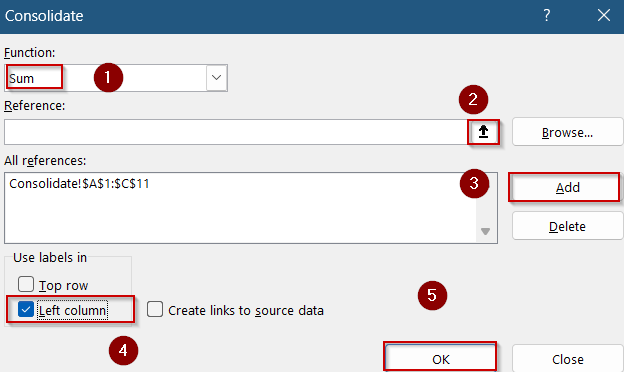
➤ In the Function dropdown, select Sum to total the sales.
➤ In the Reference box, select your full dataset (A1:C11) and click Add.
➤ Check both Top row and Left column or either of them to let Excel use your headers for grouping.
➤ Click OK.
Excel will generate a summary that shows the total Sales per unique Product in the selected output range.
Note:
This approach groups by the first column only (in this case, Product). It does not support grouping by multiple fields like Product and Region.
Insert the UNIQUE Function to Return Distinct Rows
The UNIQUE function in Excel 365/2021 dynamically pulls only distinct rows from a range. It’s ideal for cleanly extracting unique records based on entire rows, not just one column. This array formula updates automatically when you add or remove rows in the original dataset, making it perfect for reports or dashboards that require live data filtering.
Steps:
➤ Click on a blank cell (e.g., E2).
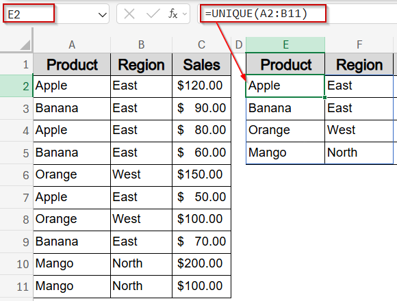
➤ Enter the following formula to return unique rows:
=UNIQUE(A2:C11)
➤ Press Enter, and Excel will immediately return each unique Product and Region combination.
➤ To sum the Sales for each unique combination, enter this formula in cell G2:
=SUMIFS(C2:C11, A2:A11, E2, B2:B11, F2)
➤ Drag this formula down alongside the unique rows.
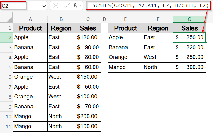
Now you have successfully merged all duplicate rows in Excel.
Create a PivotTable to Summarize and Group Duplicate Entries
PivotTables are one of Excel’s most powerful tools for summarizing data, especially when dealing with duplicate rows that need to be grouped and analyzed. Unlike static tools, PivotTables are dynamic as they automatically update when your source data changes, and they can be grouped by multiple columns like Product and Region. This makes them perfect for calculating total sales, counting entries, or spotting trends across categories.
Steps:
➤ Click anywhere inside your dataset to activate it (e.g., any cell in A1:C11).
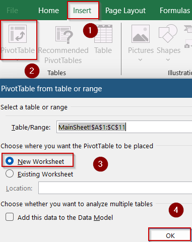
➤ Go to the Insert tab on the Ribbon and click PivotTable.
➤ Choose whether to place the PivotTable in a new worksheet or in an existing sheet and click OK.
➤ In the PivotTable Fields pane on the right, drag Product to the Rows area to group data by product name and drag Sales to the Values area and Excel will automatically sum the values.
➤ Optionally, drag Region to the Rows area below Product to break totals down by region.
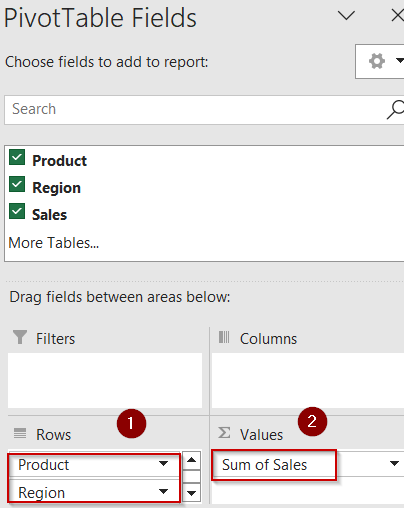
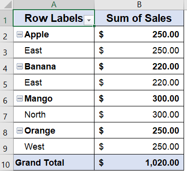
Excel will instantly generate a clean, structured table showing the total sales per product, and optionally by region to automatically merge all duplicates in the process.
Automate Merging and Summing Duplicates Using Power Query
Power Query is an advanced yet beginner-friendly tool in Excel that helps streamline data cleanup tasks like merging duplicates and summing related values. This method is perfect for large or dynamic datasets where you want to automatically combine duplicate rows (e.g., by product name) and calculate total sales, all while keeping the results refreshable. Once set up, you can reuse this query anytime with just one click to update your data.
Steps:
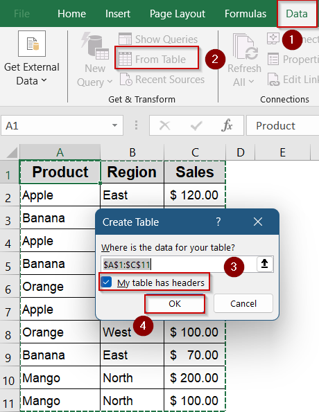
➤ Select your dataset including headers >> Go to the Data tab >> Click From Table/Range (Excel will convert your range into a table if it isn’t already).
➤ If prompted, confirm that your table has headers and click OK to open the Power Query Editor.
➤ In the Power Query Editor, click on the Product column to highlight it.
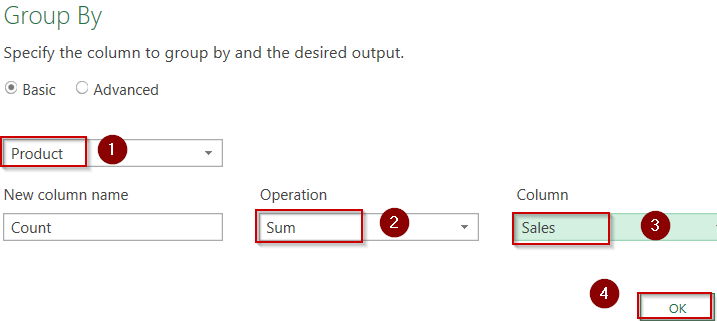
➤ Go to the Home tab in Power Query >> Click Group By in the ribbon.
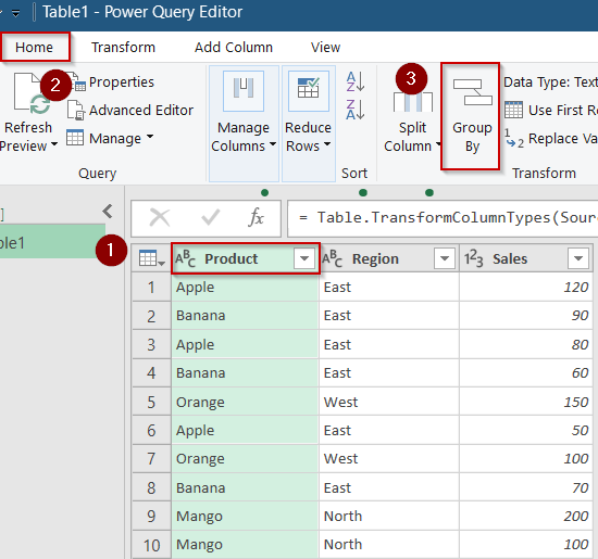
➤ In the Group By window that appears, set Group by to Product, Operation to Sum, and Column to Sales.
➤ Click OK to apply grouping and summing.
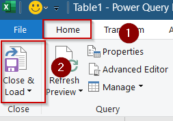
➤ Now go to the Home tab again >> Click Close & Load to send the transformed data back to your Excel sheet.
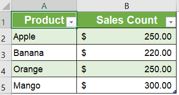
You’ll now see a brand-new table with duplicates merged by product and the total sales summed and any future changes to your original data can be updated simply by refreshing the query.
Run VBA to Merge Duplicate Rows and Sum Corresponding Values
If you’re working with a large dataset and want to automatically merge rows based on a common key (like product name) while summing values across multiple columns, this VBA macro provides a fast and customizable solution. Unlike PivotTables or Consolidate, VBA gives you full control over the logic and allows you to output the cleaned data anywhere in your workbook without overwriting the original data. This is ideal when you want to summarize data programmatically and apply it to multiple sheets or reports with minimal effort.
Steps:
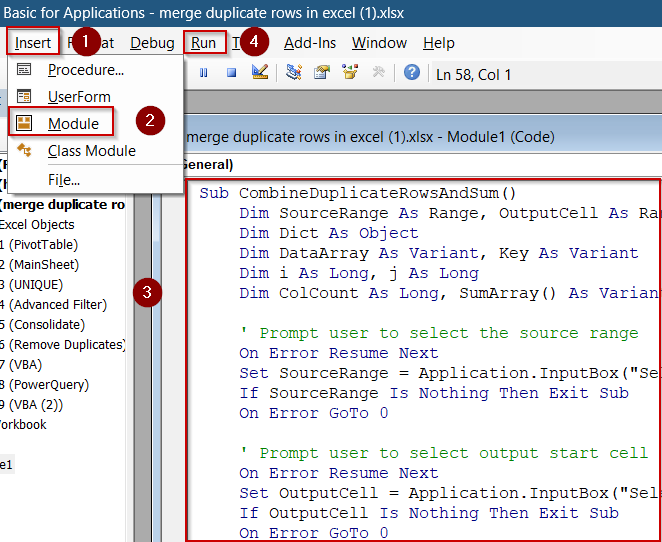
➤ Press Alt + F11 to open the VBA Editor.
➤ Click Insert >> Module to create a new module.
➤ Paste the following code into the module:
Sub CombineDuplicateRowsAndSum()
Dim SourceRange As Range, OutputCell As Range
Dim Dict As Object
Dim DataArray As Variant, Key As Variant
Dim i As Long, j As Long
Dim ColCount As Long, SumArray() As Variant, TempArray As Variant
' Prompt user to select the source range
On Error Resume Next
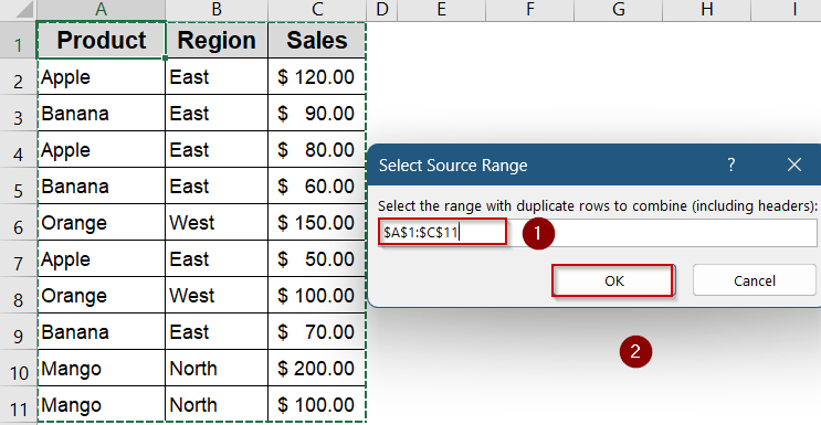
Set SourceRange = Application.InputBox("Select the range with duplicate rows to combine (including headers):", "Select Source Range", Type:=8)
If SourceRange Is Nothing Then Exit Sub
On Error GoTo 0
' Prompt user to select output start cell
On Error Resume Next
Set OutputCell = Application.InputBox("Select the starting cell to output the result:", "Select Output Cell", Type:=8)
If OutputCell Is Nothing Then Exit Sub
On Error GoTo 0
' Initialize variables
Set Dict = CreateObject("Scripting.Dictionary")
DataArray = SourceRange.Value
ColCount = SourceRange.Columns.Count
' Process each row
For i = 2 To UBound(DataArray, 1) ' Start from row 2 to skip header
Key = DataArray(i, 1)
If Not Dict.Exists(Key) Then
ReDim SumArray(1 To ColCount - 1)
For j = 2 To ColCount
SumArray(j - 1) = DataArray(i, j)
Next j
Dict.Add Key, SumArray
Else
TempArray = Dict(Key)
For j = 2 To ColCount
TempArray(j - 1) = TempArray(j - 1) + DataArray(i, j)
Next j
Dict(Key) = TempArray
End If
Next i
' Output headers
For j = 1 To ColCount
OutputCell.Cells(1, j).Value = DataArray(1, j)
Next j
' Output results
i = 2
For Each Key In Dict.Keys
OutputCell.Cells(i, 1).Value = Key
For j = 1 To ColCount - 1
OutputCell.Cells(i, j + 1).Value = Dict(Key)(j)
Next j
i = i + 1
Next Key
End Sub
➤ Press F5 key to run the macro or click Run.
➤ Press Alt + Q to close the editor.
➤ Select your original dataset A1:C11 when prompted and click OK.
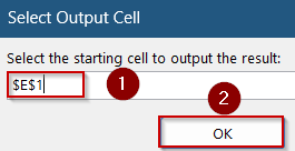
➤ Select the output cell where the results should appear such as E1 and click OK.
➤ Optionally, format your data as you prefer.
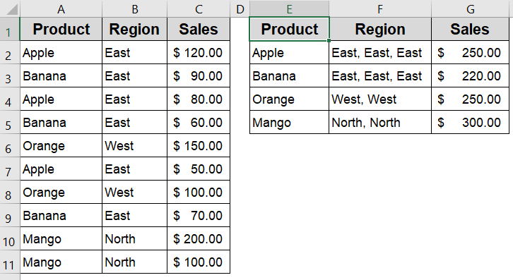
Excel will generate a new summary that merges rows with the same product name and sums the corresponding sales values, leaving your original data untouched.
This macro assumes your key column is in the first column (e.g., Product). Modify the code if you want to merge based on a different column or multiple fields.
Frequently Asked Questions
What’s the best method for large datasets?
For large or frequently changing datasets, Power Query and VBA macros are the most efficient. They automate deduplication and merging processes, can handle thousands of rows seamlessly, and reduce manual errors compared to traditional methods.
Can I merge duplicates based on multiple columns?
Yes, you can merge or remove duplicates by considering multiple columns such as Product and Region simultaneously. Tools like PivotTables, and Power Query support multi-column criteria to identify and group duplicates effectively.
Do any of these methods preserve original data?
Techniques like PivotTables, Power Query, and formulas leave the original data untouched by creating separate summaries or transformed outputs. In contrast, VBA macros often modify data in-place, so backing up beforehand is important.
Can I merge duplicates and keep text values from other columns?
Yes, but it requires advanced techniques. Power Query’s “Text.Combine” function or a custom VBA macro can concatenate text fields from duplicate rows, unlike basic tools which generally only remove duplicates or sum numeric values.
Why isn’t “Remove Duplicates” summing values?
The Remove Duplicates feature only deletes duplicate rows and doesn’t perform calculations. To sum or combine values, use PivotTables, the Consolidate tool, or Power Query, which support aggregation alongside deduplication.
Wrapping Up
In this tutorial, we explored multiple practical ways to merge duplicate rows in Excel ranging from simple tools like Consolidate and PivotTables to more advanced options like Power Query and VBA. Each method serves a different purpose depending on whether you want to keep, combine, or summarize data from repeated entries. Feel free to download the practice file and share your feedback.