
In our Excel dataset, we often encounter blank values or text values. Including the blank value on average can yield misleading results, while including the text data will return an error. Thus, to avoid such cases and get accurate results, we need to average only cells with values. For this purpose, we can use the AVERAGE and AVERAGEIF functions. In this article, we will explain the methods to use these two functions.
➤ First, select cell D1 and write a suitable name for the later calculation.
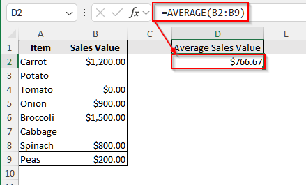
➤ Then, click on cell D2 and insert the following formula:
=AVERAGE(B2:B9)
Here, remember to replace the cell range (B2:B9) with your dataset cell range.
➤ Finally, press Enter, and it will return the average of only cells with numerical values except zero and blanks.
Calculate Average of Cells with Only Values in Excel With the AVERAGE Function
The AVERAGE function ignores all non-numeric values and calculates the average only for the numeric values, like 0, 1, 2, etc.
We will use the dataset below to explain how the AVERAGE function calculates the average of cells with only numeric values in Excel.
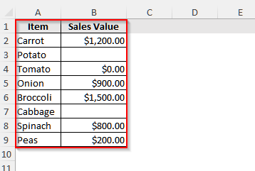
This is a sales dataset for a grocery store from a specific date. Here, we can see that some items’ sales value is zero as no one bought them, and some items are blank as those items were not available that day. To make sure the average revenue of that day is accurate, we need to calculate the value ignoring the blanks and zeroes.
Steps:
➤ First, click on cell D1 and write Average Sales Value.
➤ Then, select cell D2 and insert the following formula:
=AVERAGE(B2:B9)
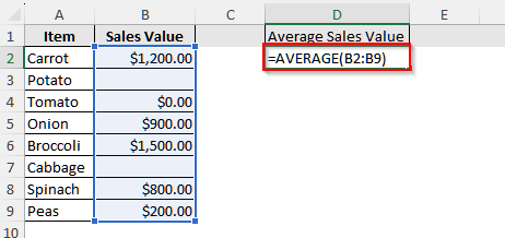
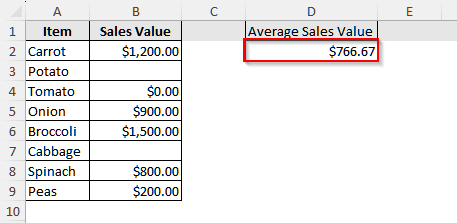
➤ Finally, press Enter, and you will see the average value of the cells with values only.
AVERAGEIF Function to Average Cells With Values Only in Excel
When we need to calculate the average for a certain group or need to apply a certain condition, we use the AVERAGEIF function. By default, this function excludes blank cells. However, if we need to exclude zero or any other values, we need to include the condition in the argument of the function. Let’s take a look at how this function works.
We will use the dataset below to explain how the AVERAGEIF function works.
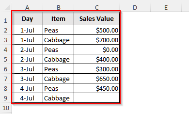
This is a dataset of four days of a grocery store for only two items, peas and cabbage. In this dataset, we can see that on 2nd July nobody bought peas, and on 4th July cabbage was not available, thus it is blank. Using the AVERAGEIF function, we will calculate the average sales value of these two items separately, ignoring the blanks and zeros.
Steps:
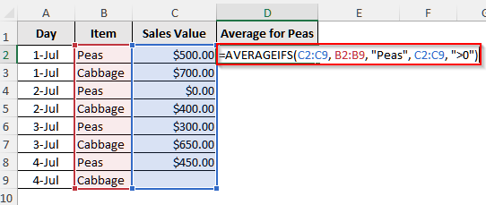
➤ First, select cell D1 and write Average for Peas.
➤ Then, click on cell D2 and insert the following formula:
=AVERAGEIFS(C2:C9, B2:B9, "Peas", C2:C9, ">0")

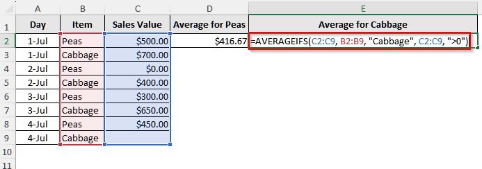
➤ Now, press Enter, and you will see the average sales value of peas for only the cells with values.
➤ Again, for cabbage, select cell E1 and give it a name.
➤ Now, click on cell E2 and insert the given formula:
=AVERAGEIFS(C2:C9, B2:B9, "Cabbage", C2:C9, ">0")
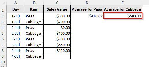
➤ Finally, press Enter,r, and it will return the average sales value for cabbage, ignoring any zeros and blanks.
Frequently Asked Questions
Can I Average Only Cells With Values for a Certain Date?
Yes, using the AVERAGEIF function, you can do it. Suppose you have Jul-1 to Jul-4 dates in column A and sales value in column B. Now, to average the sales value of Jul-2, insert the following formula in any blank cell: =AVERAGEIFS(B:B, A:A, “Jul-2”, B:B, “<>”). Now, press Enter, and you will see the average value of Jul-2.
Can I Calculate the Average for Partial matches of Cells With Only Values?
Absolutely. With the AVERAGEIF function, you can easily calculate the average for partial matches and ignore zero, blank, or any value you want. Let’s say we have three types of peas under items in our dataset, including sweet pea, green pea, and pea mix. The items are in column A, and the sales value is in column B. Now, to calculate the average sales value of peas, insert the following formula in a blank cell of the dataset: =AVERAGEIFS(B:B, A:A, “*Pea*”, B:B, “>0”). Here, the character “*” acts as a wildcard.
How to Calculate Average Excluding a Certain Group or Item?
To calculate the average excluding a certain group ot item, we need to use the AVERAGEIF function. Suppose we have a dataset where in column A we have a few items, including banana, apple, guava, grapes, etc., and in column B we have the sales value. Now, if you want to calculate the average sales value excluding Apple, insert this formula in a blank cell: =AVERAGEIF(A:A, “<>Apple”, B:B).
Wrapping Up
In this article, we have learned to calculate the average in Excel with the AVERAGE and AVERAGEIF functions for only cells with values. We have also explained how to calculate the average for a certain item or group using the AVERAGEIF function. Try these methods yourself and reach out if you have any queries.