How to Calculate Average in Excel Ignoring #N/A Error

If we try to calculate the average of a range of data in Excel that contains NA or #NA, it will return an error instead of any value. Thus, we need to ignore this NA or #NA while calculating the average. For this purpose, we can use the AVERAGEIF and AGGREGATE functions.

In this article, we will explain how to use both of these functions to ignore NA or #NA values while calculating the average in Excel.

The AVERAGEIF function allows us to use conditions within its argument, and therefore, we can modify the condition to ignore the NA error from our selected range. Let’s take a look at how we can do this.

To explain how to calculate the average in Excel, ignoring NA using the AVERAGEIF function, we will use the dataset below.

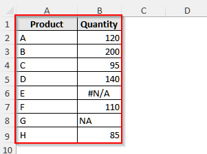
This is a product quantity demo dataset where products E and G are not available and thus represented by #N/A and NA.  We will calculate the average quantity of these products, ignoring these two unavailable ones.

Steps:

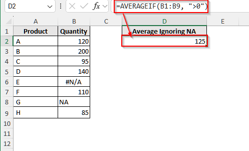
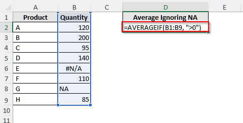
➤ First, click on cell D1 and write Average Ignoring NA.
➤ Then, select cell D2 and insert the following formula:

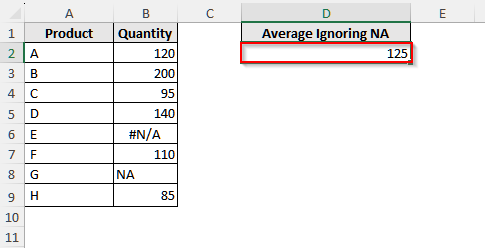
➤ Press Enter, and it will return the average value of the selected range, ignoring both NA values and #N/A errors.

Though the AVERAGE function can help us to calculate average ignoring both NA values and #N/A error, it cannot include any negative values while doing so. Thus, we need to use another method if our data has both of these issues while it contains negative values. For such cases, the AGGREGATE function is our best choice.

We will use the below dataset to show how to use the AGGREGATE function to calculate average, ignoring NA and #N/A in case of dataset contains negative values.

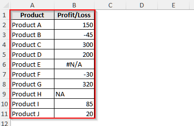
This is a profit and loss dataset for a few products of a store, which contains NA values, #N/A errors, and negative values. Let’s take a look at how we can tackle such a situation and calculate the average properly.

Steps:

➤ First, select cell D1 and give it a suitable name.
➤ Then, click on cell D2 and insert the following formula:

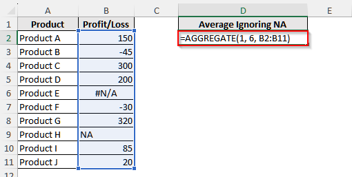
Here, the first argument, 1, represents average, the second argument, 6, indicates to ignore any error value, and the last argument, B2:B11, is the selected range.

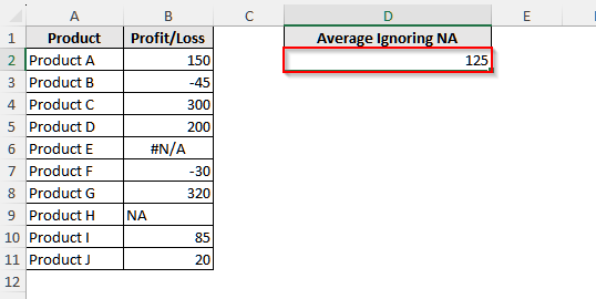
➤ Now, press Enter on your keyboard, and it will return the calculated average.

Frequently Asked Questions

How to Calculate Average if My Data Has Only #N/A Error?

If your data has only #N/A errors, use the AVERAGEIF function to calculate the average. Suppose you have data in column B from B2 to B10. Then, insert the following formula in any blank cell: =AVERAGEIF(B2:B10,”<>#N/A”). It will return the average value, ignoring the #N/A error.

Why Cannot I use the AGGREGATE Function?

If your Excel is an older version or a limited version, you cannot use the AGGREGATE function. In such a case, to calculate the average ignoring NA for data with negative values, you need to use a modified version of the AVERAGE function. Suppose the data is in column B from range B2 to B10. Then, enter the following formula in a blank cell: =AVERAGE(IF(NOT(ISNA(B2:B10)), B2:B10)). If this formula does not work, you need to press  Ctrl  +  Shift  +  Enter  instead of only  Enter  .

How Can I Average Non-Contagious Cells in Excel Ignoring NA Error?

You can average non-contagious cells using both AGGREGATE and AVERAGE  functions. Let’s say you have data in column B in cells B2, B4, and B7. Now, if your Excel supports the AAGGREGATE function, insert the following formula, =AGGREGATE(1, 6, (B2, B4, B7)) in a blank cell, and it will return the average value. Also, if your data has any NA error value, do not include the cell reference inside this formula. Such as, If B8 is an NA error, just ignore this cell reference in your formula.

Also, if your Excel does not support the AGGREGRATE function, use this formula instead: =AVERAGE(IF(NOT(ISNA(B2)), B2, “”), IF(NOT(ISNA(B4)), B4, “”), IF(NOT(ISNA(B7)), B7, “”)). It is an array formula, and so you need to press  Ctrl  +  Shift  +  Enter  instead of only  Enter  .

Wrapping Up

In this article, we have learned to calculate the average in Excel, ignoring both NA values and #N/A error using the AVERAGEIF and AGGREGATE functions. We also learned that in case of negative values, we need to use the AGGREGATE function as the AVERAGEIF function cannot calculate the average in such a situation, while ignoring both NA and #N/A errors. Give these methods a try and reach out if you have any queries.