How to Search Data in Google Sheets

When working with data management, analysis, and organization, you can work more quickly and efficiently by managing your data in Google Sheets. But you need to know how to search properly. Working with large datasets provides precise information and saves time. You can easily find phrases, figures, or patterns in your spreadsheet by searching in the right way. In this article, we will describe the process of finding a single value, the highest value, the first cell with a value, searching for a word in a shortcut way and many more ways to search in Google Sheets

Search for a Word Using Keyboard Shortcut in Google Sheets

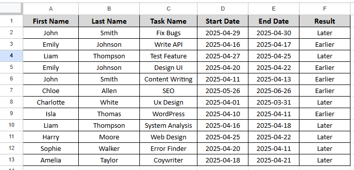
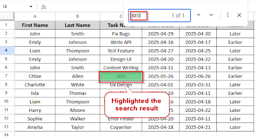
When you’re working with lots of data in Google Sheets, you need to search for a specific word to save your time. Using a keyboard shortcut, you can search for a word easily on Google Sheets. Let’s look at the dataset below, where you want to search for the “SEO” word. Follow these instructions step by step to search in a shortcut way.

➤ Press  Ctrl  +  F  for windows or  Cmd  +  F  on Mac. A small search bar will appear in the sheet.

➤ Type the word “SEO”. Google Sheets will highlight all matching words in the current sheet

Search for a Text in a Range and Extract Rows with the FILTER Function

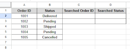
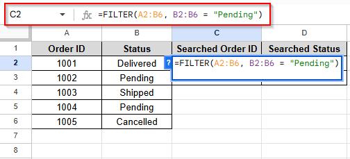
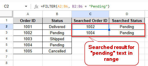
When working with a larger dataset, you need to search for text within a defined range. There is no “search in range” button in Google Sheets. But you can easily search for text by using built-in functions. By using functions, you can search for specific text in a range in Google Sheets. Let’s look at the dataset below, where you want to search for Status = “Pending” in a row. Follow these instructions step by step to search for text in a range.

➤ Click on cell C2 and write this formula :

➤ Press Enter and see the search result.

Search All Sheets in Google Sheets

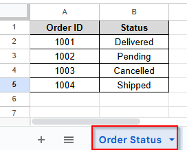
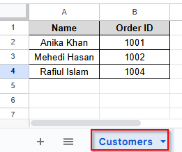
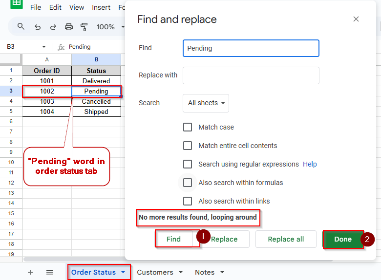
When you have multiple sheets in Google Sheets, you want to search for a specific word. You can search across all sheets at once by using the “find and replace” tool in Google Sheets. Let’s look at the three datasets( order status, customers and notes) below, where you want to find the “pending” word across all sheets at once. Follow these steps to search all sheets in Google Sheets.

➤ Press  Ctrl  +  H  (Windows) or  Cmd  +  H  (Mac) to open the find and replace window. In the Find field, type: Pending. Click Find to jump to each match one by one. You can see the first result in the notes tab.

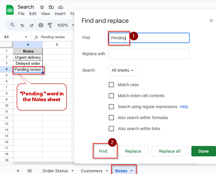
➤ Click the “Find” Button again, and you can see another finding result across the sheets. When there are no results, you can see the text “ no more results found, looping around”.

Find All Cells with a Specific Value in Google Sheets

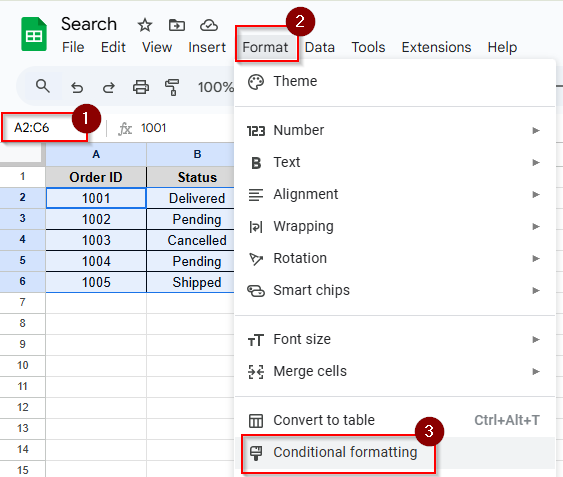
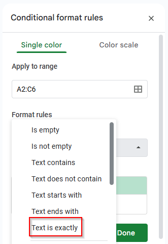
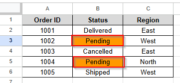
You can find all cells that contain a specific value in Google Sheets. Then you can highlight those values in Google Sheets. It’s so helpful when you are working with larger datasets. Let’s look at the dataset below, where you want to find the “ Pending” value in all cells. Follow these steps to find all cells with a value that contains “pending”

➤ Select the cells A2:C6 and click Format > Conditional Formatting

➤ In the conditional formatting rules option, click Format Cells if and then click the arrow.

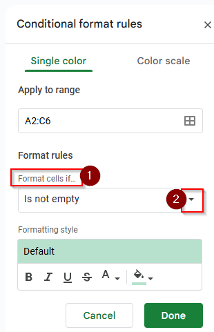
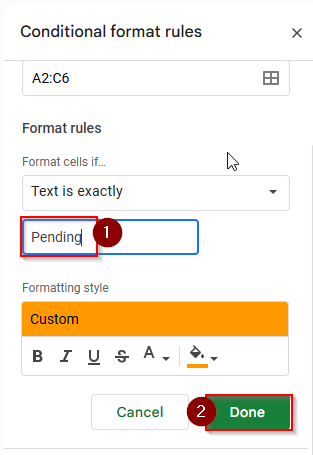
➤ Choose the “Text is Exactly” option from the dropdown menu

➤ Write “ Pending” in the text box and click Done. You can customize the color in the formatting style option.

➤ Now you can see the result, the Pending word is found and highlighted

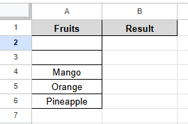
Find Merged Cells in Google Sheets

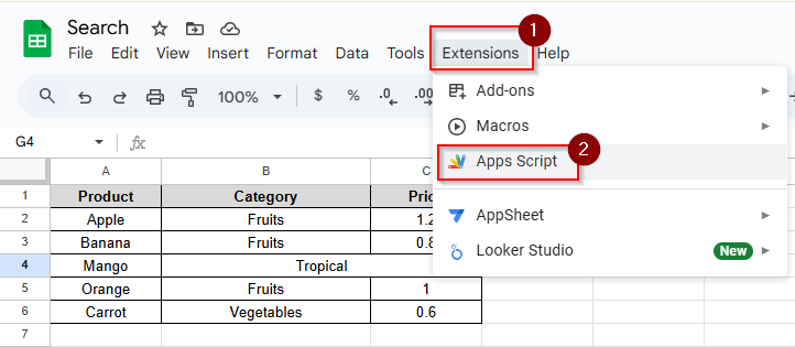
You can find which cells are merged in Google Sheets. Finding merged cells is very important because it can cause problems with sorting, filtering, or data analysis. You can find it manually by looking at the dataset. You can do it with Apps Script code. Let’s look at the dataset below, where you want to find the merged cells. Follow these instructions to find it with Apps Script.

➤ Click Extensions > Apps Script

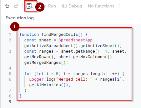
➤ Paste the following code in the Apps Script and click the Save icon

function findMergedCells() {
  const sheet = SpreadsheetApp.getActiveSpreadsheet().getActiveSheet();
  const ranges = sheet.getRange(1, 1, sheet.getMaxRows(), sheet.getMaxColumns()).getMergedRanges();
for (let i = 0; i < ranges.length; i++) {
 Logger.log("Merged cell: " + ranges[i].getA1Notation());
  }
}

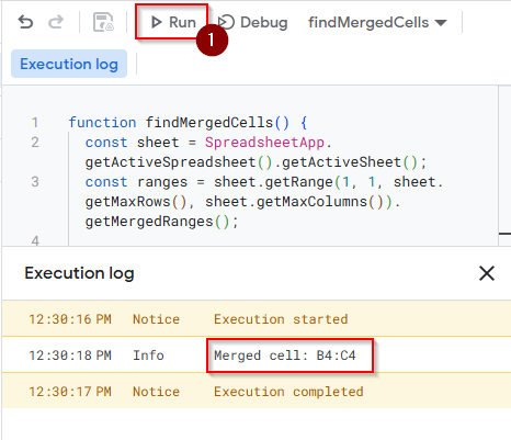
➤ Click the Run option to run this code in the execution log. You can see the result below. Merged cell: B4:C4

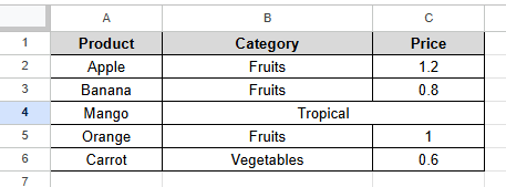
Find First Cell With Value in Google Sheets

When you are working with a dataset that contains the first cell with a blank and you need to find out the first cell that contains any value, you can do this by using a formula. You can find the cell number and see the value. Follow these instructions to see which cell contains a value.

➤ Click on cell B2 and write this formula:

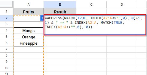
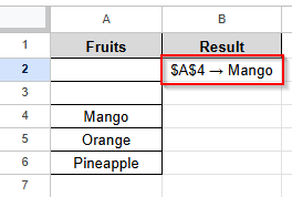
➤ You can see the result. First A4 cell contains the value mango.

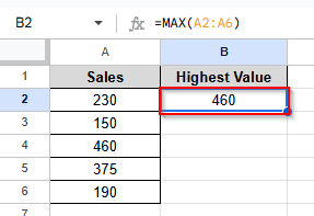
Find the Highest Value in Google Sheets

You need to find the highest value in Google Sheets for analyzing sales, scores, prices, or any numerical data. You can find the highest value in a dataset by using the MAX function. Follow these steps to find the highest value in Google Sheets.

➤ Click on cell B2 and write this formula:

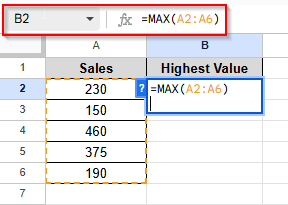
➤ Press Enter and see the highest value of this dataset. The highest value is 460.

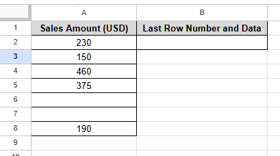
Find the Last Row with Data in Google Sheets

When you’re working with dynamic data or want to avoid blank rows, you need to find the last rows that contain any data in Google Sheets. Using a formula, you can find the last row number and see the data in the last row. Follow these instructions to find the last row with data.

➤ Click on cell B2 and write this formula:

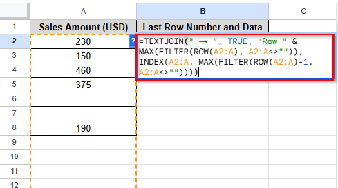
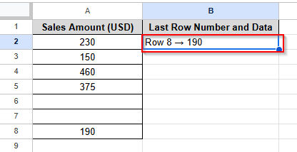
➤ Press Enter and see the result. The last row number is 8, and it contains the data 190.

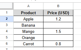
Find and Replace Blank Cells in Google Sheets

You can find the blank cells and replace those blank cells with a specific value, like “ N/A”, 0, “Missing” or anything else. This method is useful for cleaning up datasets before analysis or sharing. Let’s look at the datasets below, where there are blank cells and you want to replace those cells with N/A.

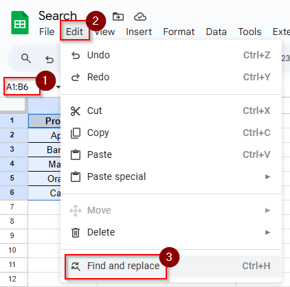
➤ Select the cells A1:B6 and click Edit > Find and Replace

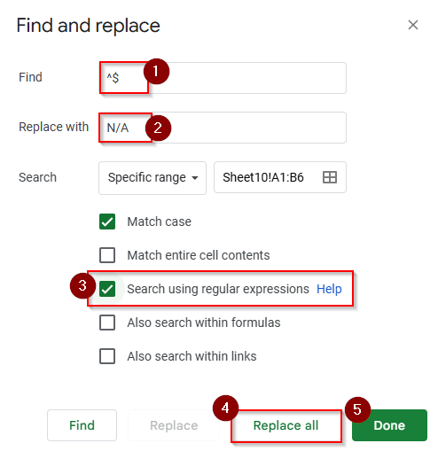
➤ In the Find and Replace box, type ^$ in the Find box, Replace with section, type N/A. Put a tick mark in the Search using regular expressions. Click the Replace All button and then DONE.

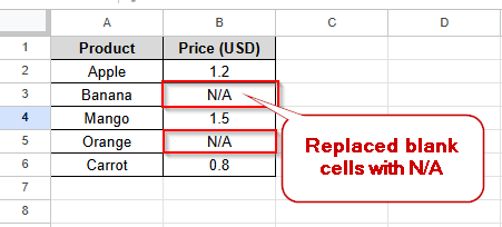
➤ Now see the result in the dataset. Blank cells in the B3 and B5 are replaced with N/A.

Frequently Asked Questions

Is there any way to search case-sensitive text?

In the Find and Replace window, put the tick mark in the Match case box. Only exact matches case case-sensitive text will be found in the search result.

Is it possible to highlight cells that have a specific word?

Of course. Select conditional formatting under the format option, and then apply the rule. Enter the keyword in the text. You can highlight cells that contain a specific word.

Concluding Words

Searching in Google Sheets is simple, but it is very important to save your time and keep your data clean, organized. You can search very easily using  Ctrl  +  F  to find a word. With a few clicks or calculations, you can find specific values, blank cells, merged ranges, or even the last data in a dataset. We described in detail the search ways in Google Sheets. If you have any questions or get stuck in any step, feel free to share with us in the comment section.