The AVERAGEIF function in Excel is used to calculate the average of numbers that meet a single condition. For example, you might want to find the average sales amount for a specific region or product. It’s a simple way to filter and average values in one step.
However, sometimes one condition isn’t enough. You may want to calculate the average only for values that meet multiple criteria, such as sales greater than zero, delivered before a certain date, and from a specific region.
In these cases, Excel’s built-in functions like AVERAGEIFS, or a combination of SUMIFS and COUNTIFS, give you the flexibility to apply more than one condition.
In this article, you’ll learn how to use AVERAGEIF formulas with multiple criteria in Excel.
We’ll use the AVERAGEIF function to find the average sales amount for products that have sales greater than 0, are in the North region, and were delivered on or before 30-Oct.
Here’s how to do it:
➤ Open your dataset in Excel.
➤ Click on the cell where you want to display the result. In our example, this is cell G5.
➤ Enter the following formula:
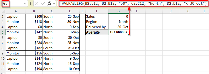
=AVERAGEIFS(B2:B12, B2:B12, “>0”, C2:C12, “North”, D2:D12, “<=30-Oct”)
➤ Press Enter.
➤ Excel will return the average sales amount for products that meet all three criteria: North region, sales above 0, and delivered by 30-Oct.
Using AVERAGEIFS to Apply Multiple Criteria
In the following dataset, we have a simple sales record that tracks different products, their sales values, regions, and delivery dates. Column A lists the Product Names, Column B contains the Sales amounts, Column C shows the Region where each sale occurred, and Column D holds the Delivery Dates.
On the right, we’ve created a criteria table where we define conditions such as minimum sales amount, region, and latest delivery date. Our goal is to calculate the average sales value for products that meet all these specified conditions.
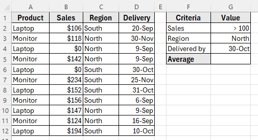
We’ll use this dataset to demonstrate how to apply multiple criteria using Excel formulas and return an accurate average based on the filtered results.
The AVERAGEIFS function is designed to calculate the average of a range based on two or more conditions. It’s the easiest and most direct way to average values that meet multiple criteria in Excel.
We’ll use this method to find the average sales amount for products that have sales greater than 0, are in the North region, and were delivered on or before 30-Oct.
Here’s how to do it:
➤ Open your dataset in Excel.
➤ Click on the cell where you want to display the result. In our example, this is cell G5.
➤ Enter the following formula:
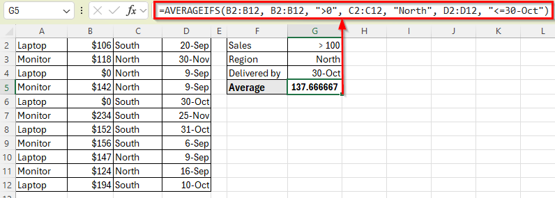
=AVERAGEIFS(B2:B12, B2:B12, ">0", C2:C12, "North", D2:D12, "<=30-Oct")
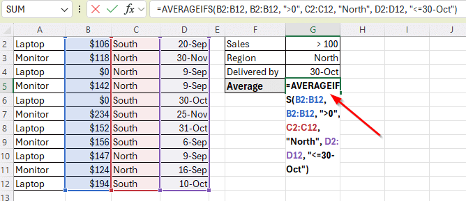
➤ Press Enter.
➤ Excel will return the average sales amount for products that meet all three criteria: North region, sales above 0, and delivered by 30-Oct.
Note:
Make sure the Delivery column is properly formatted as Date in Excel. If the dates are stored as text, the date comparison may not work correctly.
Use AVERAGE with IF for an Array Formula
Another way to calculate the average with multiple criteria is by using the AVERAGE function combined with an IF statement inside an array formula. This approach gives you full control over the logic and works well if you’re using older versions of Excel that don’t support AVERAGEIFS.
In this method, we’ll calculate the average sales for products that have sales greater than 100, are from the South region, were delivered on or before 25-Nov.
Here’s how to do it:
➤ Select the cell where you want to display the average, for example click on cell G5.
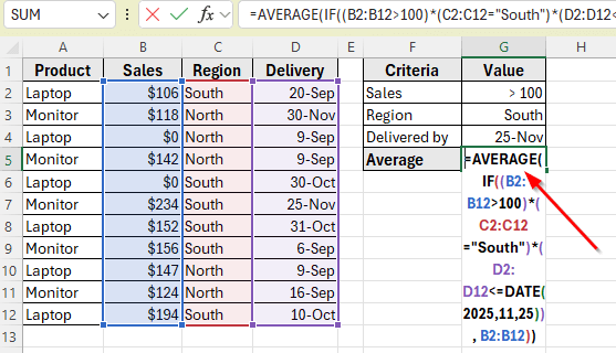
➤ Enter the following formula:
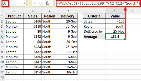
=AVERAGE(IF((B2:B12>100)*(C2:C12="South")*(D2:D12<=DATE(2025,11,25)), B2:B12))
➤ Press Ctrl + Shift + Enter if you’re using Excel 2016 or earlier.
➤ If you’re using Excel 365 or Excel 2019, just press Enter .
Alternatives to the AVERAGEIF(S) to Get Average with Criteria
Combine IF with AND Function
The AVERAGEIF function is designed to work with only one condition. It doesn’t support multiple criteria on its own. However, you can still use AVERAGEIF with multiple conditions by first combining those conditions into a helper column, and then applying AVERAGEIF to that column.
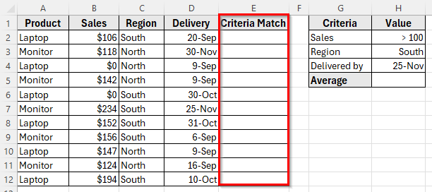
In this method, we’ll create a new column that checks whether a row meets all three criteria: sales greater than 100, region is South, and delivery date is on or before 25-Nov.
Then we’ll use AVERAGEIF to average the sales values only for rows that pass all three checks.
Here’s how to do it:
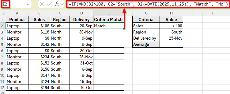
➤ In column E, label the header as Criteria Match.
➤ In cell E2, enter the following formula:
=IF(AND(B2>100, C2="South", D2<=DATE(2025,11,25)), "Match", "No")
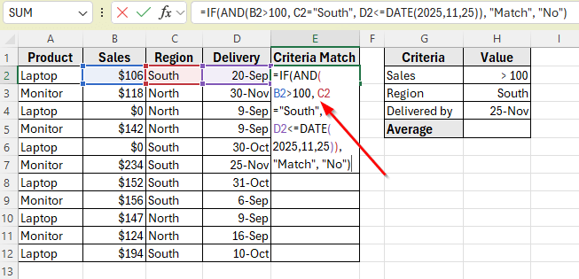
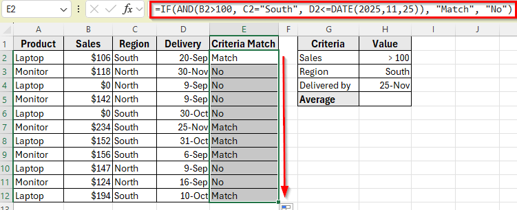
➤ Press Enter. You’ll see the result Match if the row meets all three conditions.
➤ Then drag the fill handle down to apply the formula through E12.
➤ Now, click on the cell where you want to calculate the average, for example G5.
➤ Enter this formula:
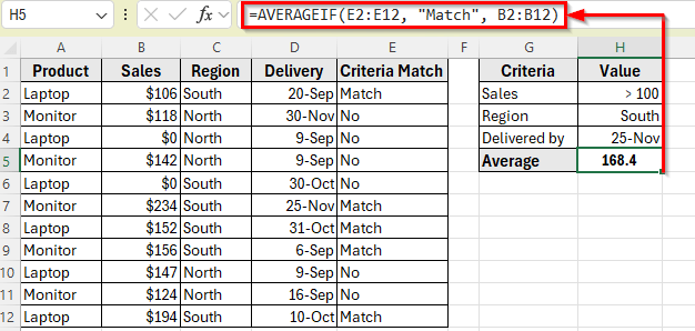
=AVERAGEIF(E2:E12, "Match", B2:B12)
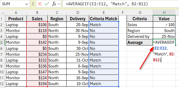
➤ Press Enter. Excel will return the average of Sales values where all three criteria are met.
Combining SUMIFS and COUNTIFS Functions
If you’re using a version of Excel that doesn’t support AVERAGEIFS, or if you want more control over the calculation, you can use a combination of SUMIFS and COUNTIFS. This manually adds up the values that meet your criteria and divides the total by the number of matching entries.
In this method, we’ll use the same conditions as before such as our sales greater than 0, the region is North, and the delivery date is on or before 30-Oct.
Here’s how to apply this method:
➤ Click on the cell G5 where you want to display the average.
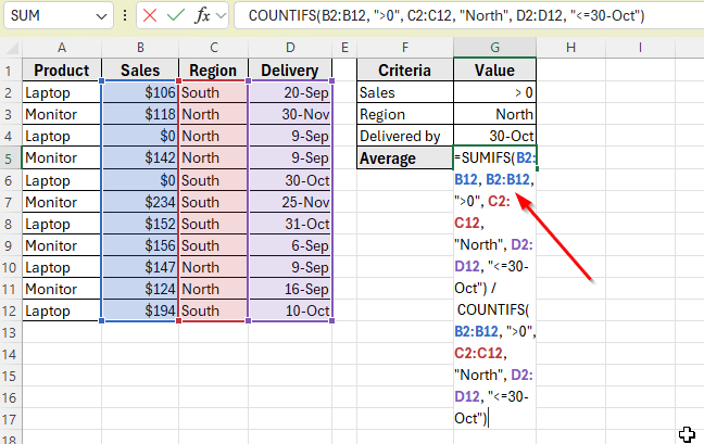
➤ Enter the following formula:
=SUMIFS(B2:B12, B2:B12, ">0", C2:C12, "North", D2:D12, "<=30-Oct") / COUNTIFS(B2:B12, ">0", C2:C12, "North", D2:D12, "<=30-Oct")
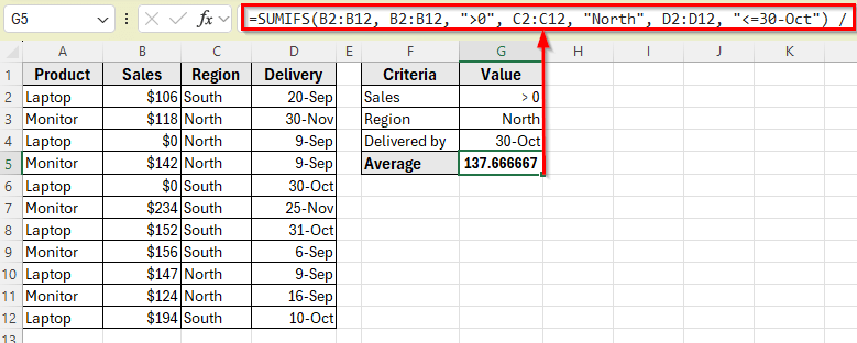
➤ Press Enter.
➤ Excel will calculate the total of all matching sales using SUMIFS, then divide that total by the count of matching entries using COUNTIFS, returning the same result as the AVERAGEIFS method.
Frequently Asked Questions
Can I use AVERAGEIF with multiple criteria in Excel?
No, the AVERAGEIF function only supports a single condition. To apply multiple conditions, you can use AVERAGEIFS, or use a helper column to combine multiple checks and then apply AVERAGEIF.
What is the difference between AVERAGEIF and AVERAGEIFS?
AVERAGEIF works with one condition, while AVERAGEIFS allows you to apply multiple criteria at once. Use AVERAGEIFS when you need more control and flexibility in your averaging logic.
What happens if no values match my criteria?
If none of the rows meet your conditions, AVERAGEIFS will return a #DIV/0! error because it’s trying to divide by zero. You can wrap the formula in IFERROR to handle this:
=IFERROR(AVERAGEIFS(…), “No Match”)
Wrapping Up
The AVERAGEIF function is useful when you want to calculate an average based on a single condition, but it becomes limited when multiple criteria are involved. In those cases, Excel offers several flexible alternatives.
The AVERAGEIFS function is the most straightforward way to apply multiple conditions at once. You can also combine SUMIFS and COUNTIFS, or use array formulas for more control. If you still prefer using AVERAGEIF, adding a helper column lets you work around its single-condition limit.
Each method works best in different situations. Choose the one that fits your dataset and Excel version. With the right formula, you can accurately calculate averages based on multiple conditions and make your data analysis more efficient.