How to Combine VLOOKUP with COUNTIF in Excel (2 Examples)

VLOOKUP and COUNTIF are two of the most powerful functions in Excel. VLOOKUP is typically used to search for a value and return a corresponding entry, while COUNTIF is used to count how many times a certain condition or value appears in a range. So, what happens when we combine VLOOKUP with COUNTIF?

Well, combining these two functions together allows you to pull data from one part of your sheet and then summarize or analyze it in another. In this guide, we’ll show you how to combine VLOOKUP with COUNTIF correctly, using practical examples. Whether you’re building dashboards or analyzing trends, this combo will help you go beyond basic lookups and counts.

In excel, we can simply combine the VLOOKUP and COUNTIF functions together to count the occurrences of a value within a dataset. VLOOKUP goes and finds a specific item for you, like an employee name. Then, COUNTIF takes that name, and counts how many times it appears in a specific list. This method is really helpful for things like counting attendance of students or employees or just seeing how many times a particular product sold once you’ve looked up its name.

So, let’s assume we’ve a dataset in Excel, containing Employee Names and their ID values. Here we’ve also another dataset that includes the employee’s ID values and their presence in different shifts seven days in a week.

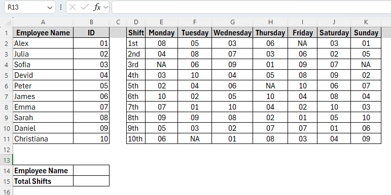
Now we’re going to count the total shifts attended by an employee named Peter using VLOOKUP with COUNTIF. Let’s see how it works.

Steps:

➤ Insert the employee name Peter in cell B14.

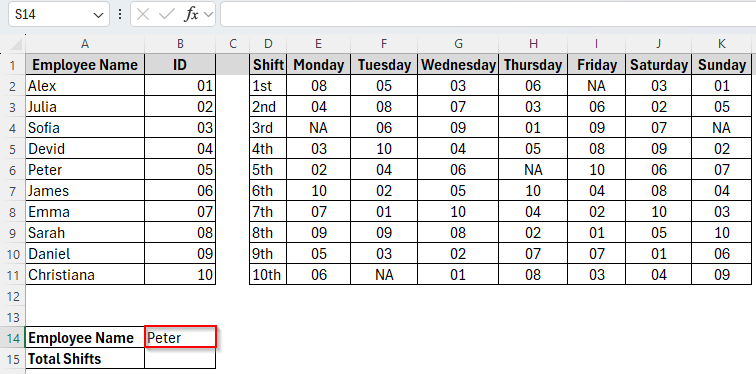
➤ Now type the following formula in the cell B15:

➤ Press Enter and here’s the result.

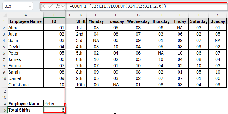
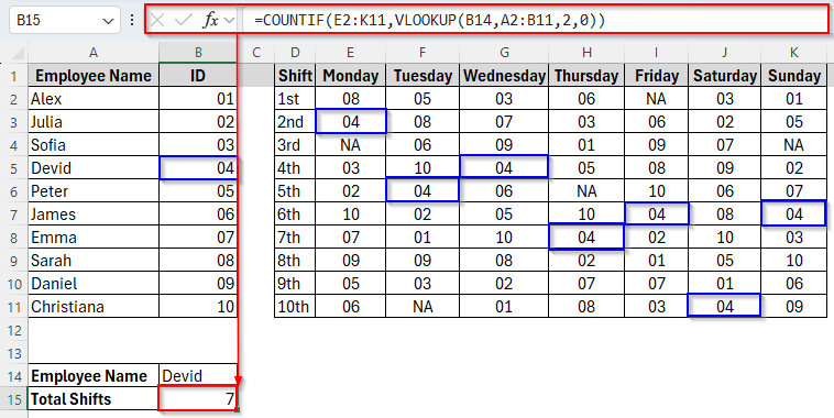
➤ We can also verify the result by counting it manually that the ID value 05 of the employee named Peter appeared 6 times in the weekly dataset.

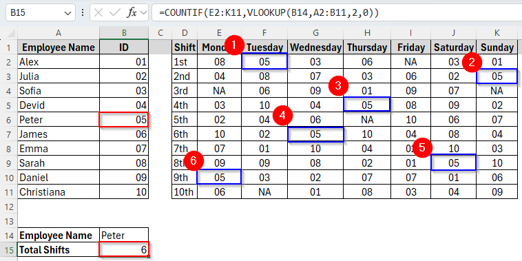
Here, VLOOKUP(B14, A2:B11, 2,0) looks up the employee name in cell B14 and returns the corresponding ID from column B. In contrast, COUNTIF(E2:K11, …) counts how many times that ID appears in the weekly shift schedule range.

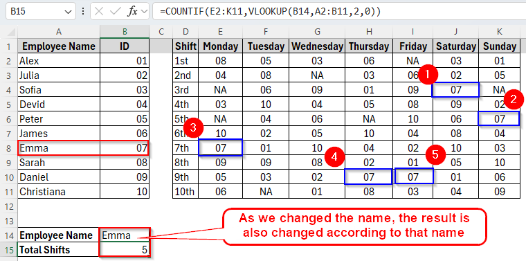
Additionally, This method is dynamic. That means changing the name in cell B14 will automatically update the total shift count in B15 using the linked ID as we can see in the image below:

In Excel, when we write formulas and copy or drag them down, Excel can automatically change the cell’s positions. For example, if we drag =A1+B1 from row 1 to row 2, it becomes =A2+B2. This is called the relative reference that Excel changes the formula to match the new row or column.

But when we combine the VLOOKUP function with the COUNTIF function, sometimes we need to lock certain parts of the formula so it stays the same no matter if we copy or drag down the formula. In this case, using the absolute reference with the dollar sign ($) would be the most effective solution. By using absolute references, we make sure the lookup range and counting range stay fixed no matter where we copy the formula.

For this, we’ve chosen another three different datasets, one including employee names and IDs, another with project assignments that contain employee IDs and the other with the employee name and number of projects attended by each employee.

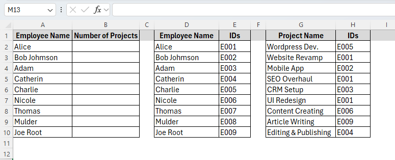
Now we’re going to count how many projects an employee named Alice has worked on using VLOOKUP and COUNTIF with the absolute references. Here’s how it goes.

Steps:

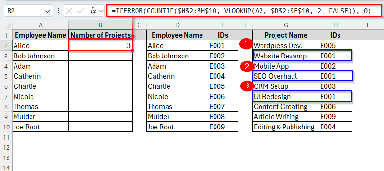
➤ Insert the following formula in the cell B2:

➤ Press Enter and you’ll get the answer as the image shows below.

➤ Now if we drag down the cell B2 to B10, we’ll also see the expected result for each employee in the list without any error.

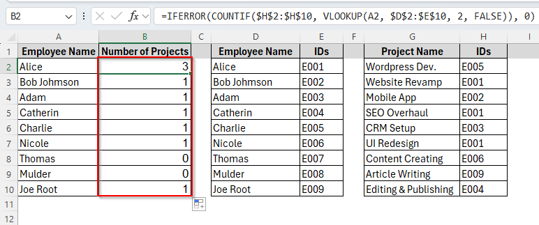
Here, in this formula, A2 mentions the employee name Alice. VLOOKUP(A2, $D$2:$E$10, 2, FALSE) looks up Alice’s ID from the Name-to-ID table and COUNTIF($H$2:$H$10,) counts how many times that ID appears in the project assignment list. We’ve also added IFERROR(…, 0) in the beginning to return 0 if the name isn’t found or no project matches.

Frequently Asked Questions

What if VLOOKUP doesn’t find the name? Will it cause an error?

Yes, normally VLOOKUP will return a #N/A error if it can’t find the name. That’s why we use IFERROR(…, 0) to catch any errors and display 0 instead of a formula error.

What happens if there are duplicate names in the lookup list?

VLOOKUP only finds the first match. So, if employee names are duplicated in your name-to-ID table, the formula may return an incorrect ID. To prevent this, make sure names are unique or use IDs as primary keys wherever possible.

Concluding Words

Combining VLOOKUP with COUNTIF is a smart and dynamic way to work with cross-referenced data in Excel. When you add absolute references and error handling, your formulas become more accurate, and ready to handle real-world datasets with ease. And if you want to take things even further, consider using XLOOKUP or INDEX-MATCH functions as more advanced alternatives.