In Excel, VLOOKUP is one of the most commonly used functions, especially for searching data. But it also has a big limitation. That is, it can only return the first match it finds in the lookup column. So what if your data has multiple matches and you want to return all of them?
While VLOOKUP alone can’t do this, there are several effective workarounds using other Excel features. In this guide, We’ll show you exactly how to return all matches using simple formulas, the FILTER function, and some other alternatives too. Whether you’re working with product lists, employee records, or repeated customer orders, this approach can help you extract full sets of matching data from large tables.
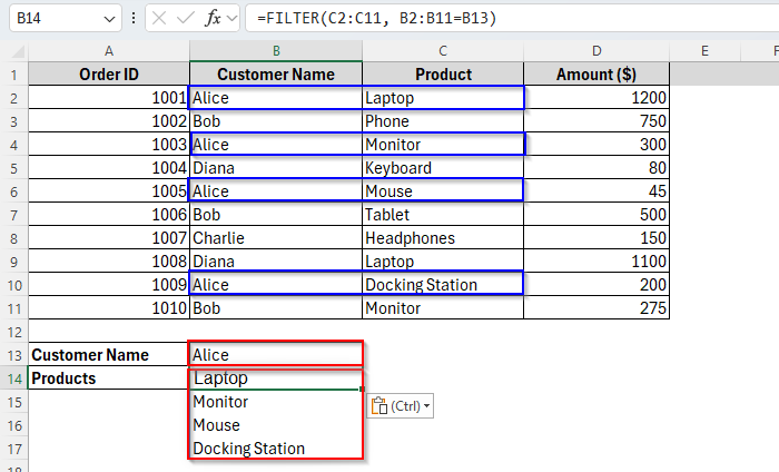
➤ Enter a customer name into cell B13.
➤ In cell B14, insert the following formula.
=FILTER(C2:C11,A2:A11=B13)
➤ Press Enter and you’ll get the result.
Now, let’s walk through step-by-step examples and explore how to apply this method with variations.
Vlookup and Return All Matches Vertically Using FILTER Function
The VLOOKUP function in Excel is great for finding out single results. But as we mentioned earlier, it cannot return all matching values in a column by default. And this is where we can simply apply the FILTER function as an alternative to VLOOKUP.
FILTER function helps you extract all matches for a given lookup value. This function filters a range of cells based on the criteria you specify. Thus it returns multiple rows or columns of data, including all matching records. It makes it perfect for creating dynamic summaries, reports, or dashboards.
So, here we’ve a Sales Record scenario with multiple orders, customer names, and the products they’ve purchased with the amount. You can see the dataset in the image below.
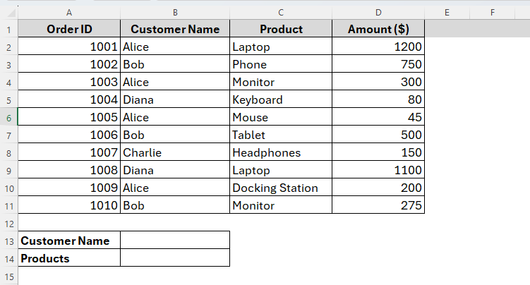
Now our goal is to return all the products bought by a specific customer from that list. Let’s say that the customer’s name is Bob. So, here’s how you can achieve it using the FILTER function, an advanced version of VLOOKUP for returning multiple results.
Steps:
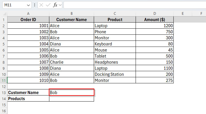
➤ Insert the customer name in cell B13.
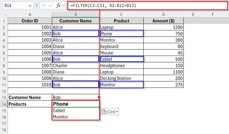
➤ Then type the following formula in cell B14:
=FILTER(C2:C11, B2:B11=B13)
➤ Press Enter, and Excel will return all matching products purchased by the customer listed in B13. These results will appear vertically, one per line, starting from B14 as the image shows below.
Vlookup and Return All Matches Horizontally Using FILTER Function
By default, the FILTER function will return all matches vertically. But what if you want to display all matching values in a single row, spread horizontally?
Well, combining the TRANSPOSE function with FILTER would be the perfect solution for this. With this method, we can simply pull all related values and display them side by side, suitable for compact reports or dashboards. Here’s how it works:
Steps:
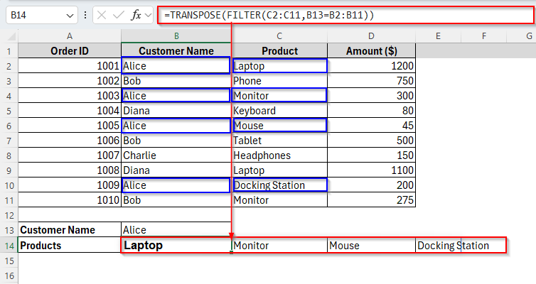
➤ Same as the previous method, type the customer name into cell B13.
➤ Then insert the following formula in cell B14:
=TRANSPOSE(FILTER(C2:C11,B13=B2:B11))
➤ Press Enter, and Excel will spill all matching product names horizontally, starting from B14 to the right.
Using Advanced Filter to Vlookup and Return All Matches
Sometimes we may need a manual but powerful way to return all matches based on a condition. That’s where we can apply Excel’s Advanced Filter. It allows you to extract all rows matching a specific value like returning all products purchased by a customer without writing formulas.
So, it’s great for users who prefer no formulas. You can get full control over what to extract, single or multiple columns. It also works well when you want to copy filtered results elsewhere. Below are the steps to follow:
Steps:
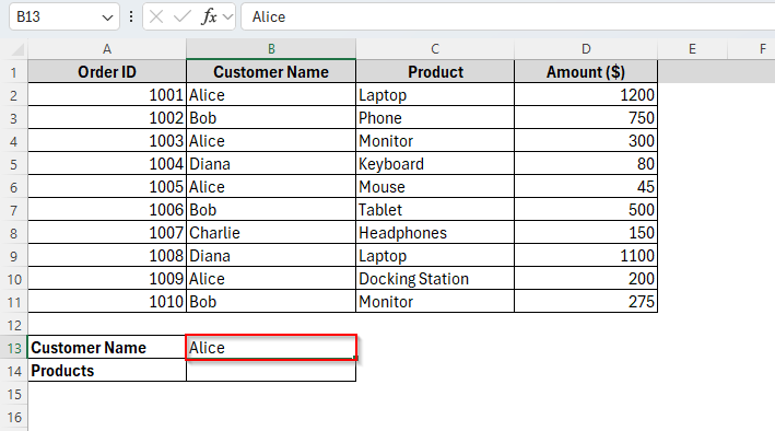
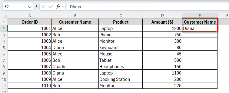
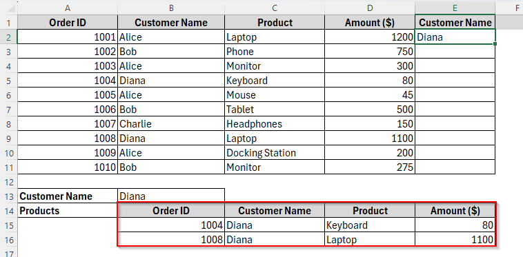
➤ In cell B13, enter the customer name Diana.
➤ Then set up a criteria range. In cell E1, type Customer Name and in cell E2, enter the same value as B13.
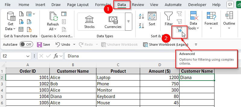
➤ Now go to the Data tab on the Ribbon and click on Advanced.
➤ Now in the Advanced Filter dialog, choose Copy to another location. Then fill up the List range: A1:D11 (your dataset), Criteria range: E1:E2 (your criteria), and Copy to: B14. and then click OK as the following image.
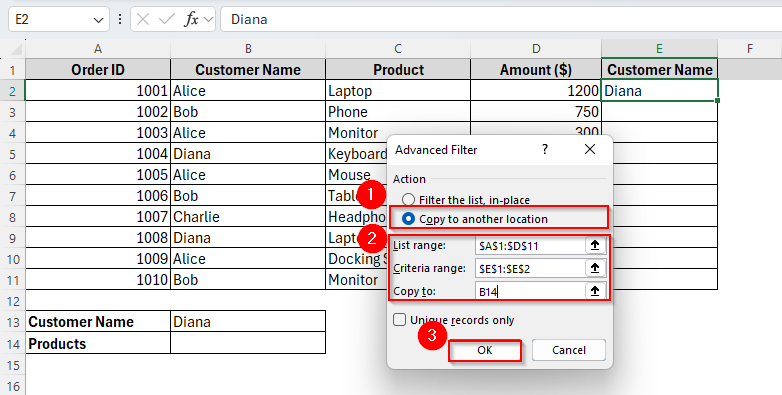
➤ Excel will now extract and display all rows where the Customer Name is Diana, including Order ID, Product, and Amount matched to this customer.
Using Power Query to Return All Matches in Excel
If you’re working with large datasets or want a reusable solution to return all matches like showing all products purchased by a specific customer, Power Query is another powerful tool available in Excel. Unlike VLOOKUP or FILTER, Power Query lets you load, transform, and filter data without writing formulas, and it’s perfect for automating repeatable tasks.
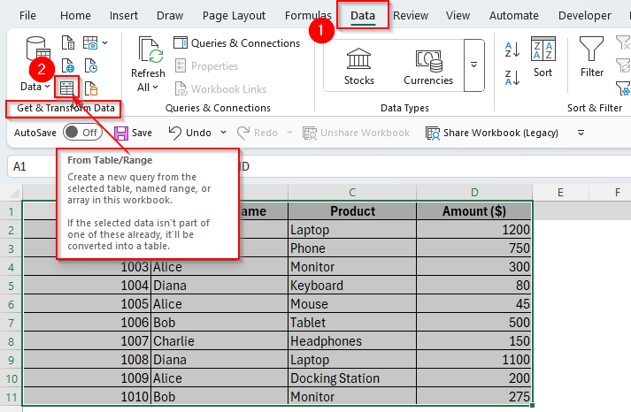
➤ To begin with, select the dataset range A1:C11 and go to Data → Get & Transform → From Table/Range
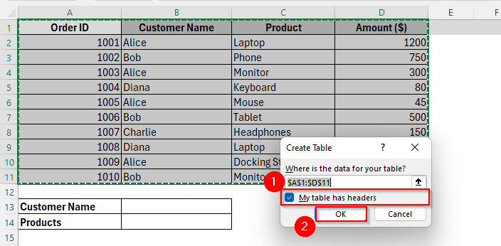
➤ In the Create Table, ensure your data has headers and then click OK.
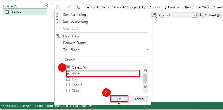
➤ In the Power Query editor, select the Customer Name column, then click the dropdown arrow → uncheck Select All and choose OK.
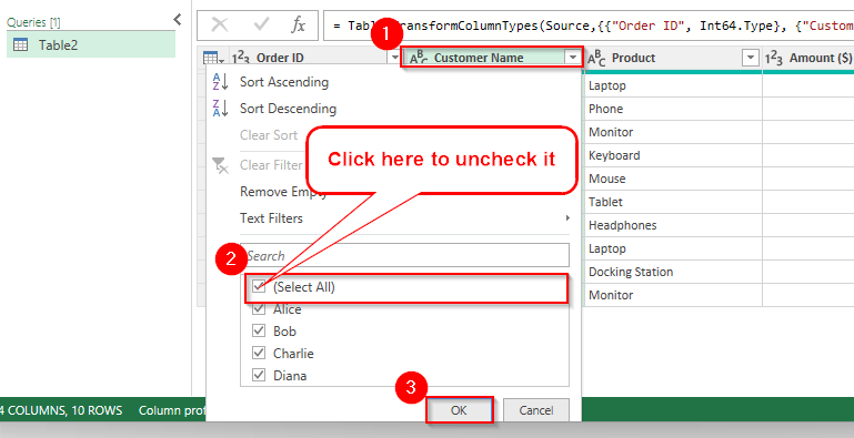
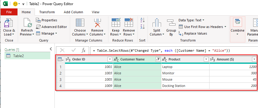
➤ Again click on the dropdown arrow and check only the customer name you want.
➤ You’ll now see only the rows where Alice is the customer.
➤ Once filtered, click Close & Load.
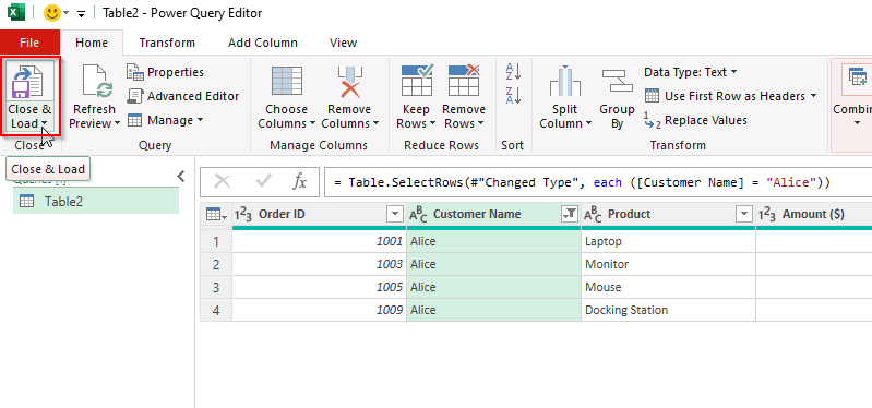
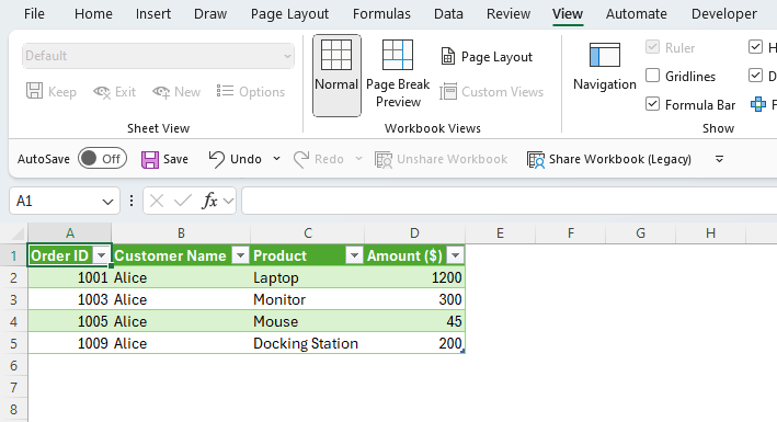
➤ It will return the filtered results to a new worksheet or table.
Frequently Asked Questions (FAQs)
What is the easiest way to return all matches?
If you have Excel 365, the FILTER function is the easiest. This will return all results from the column referred in the formula.
What if I don’t have the FILTER function?
You can use an array formula with INDEX and SMALL. It’s a bit more complex but works in older Excel versions. Another option is using Power Query to pull all matches.
Why does my VLOOKUP only show the first match?
That’s because VLOOKUP is designed to stop searching once it finds the first result. It doesn’t scan for additional matches.
Concluding Words
If you want VLOOKUP to return all matches in Excel, these are the ways you can look up and get the results. For modern users, FILTER is the cleanest solution. But for those who want a no-formula method, Power Query would be the best solution.