In data analysis, sorting the columns in a pivot table can be an important part, depending on your data. By sorting, you can organize your data properly and highlight insights that would be helpful for the managers. There are a couple of methods you can use to sort the columns in your pivot table and arrange your data.
In this article, we will show you all the methods you can use to sort the columns in your pivot table in Excel.
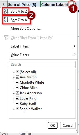
➤ Click on the dropdown arrow of the Column Labels cell of the pivot table.
➤ Choose Sort A to Z or Sort Z to A according to your choice.
Sorting columns is one of the easiest tasks in a pivot table. In this article, we will learn different methods of accessing the sorting menu and choosing your favourite sorting option for the columns. Let’s begin.
Using the Column Labels to Sort Columns in Pivot Table
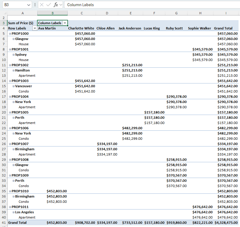
In order to explain the methods in this article, we are using a dataset of property listings. There are property IDs, cities where those properties are, property types, their prices, and the people who listed those properties for sale. The pivot table has the people’s names in the columns, the prices in the values, and everything else in the rows section. We are going to sort the names of the people in the column using different methods.
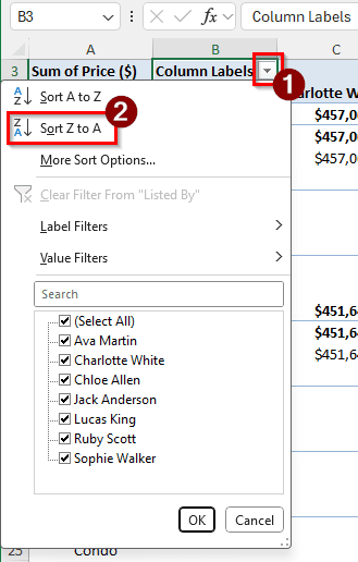
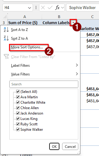
➤ At the top of the pivot table, there is a cell that says Column Labels. This cell has a dropdown button that can be used to manipulate the column names.
➤ Click on the dropdown arrow. A context menu will appear.
➤ There will be two options called Sort A to Z and Sort Z to A. Click on the second one.
Note:
If the column labels are numeric values, the options will be called Sort Smallest to Largest and Sort Largest to Smallest.
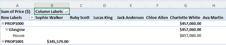
➤ The columns will be sorted from Z to A now.
Sorting from the Ribbon
In Microsoft Excel, there is a ribbon with lots of options that can be used to modify the data in the worksheet. We can use that menu to sort the columns as well. Follow the instructions below to do it:
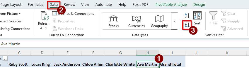
➤ Click on a column cell of the pivot table.
➤ Go to the Data tab of the ribbon menu.
➤ Find the Sort & Filter section.
➤ There will be two buttons beside the Sort button. Those buttons represent Sort A to Z and Sort Z to A buttons. Click on the lower one to Sort Z to A.
Manually Sorting the Labels
If you don’t want to sort the columns automatically, you can sort or move the labels manually, label by label. Here is the process of doing it.
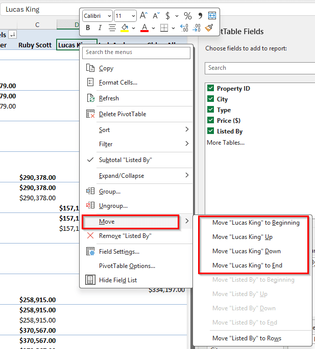
➤ Right-click on the label that you want to move.
➤ Go to Move and select where you want to move the label to.
Advanced Sorting Menu
In the other methods, we went for the general sorting system that most people will be happy with. But Excel provides us with some advanced sorting methods that we can use when required. Let’s check how to access those options.
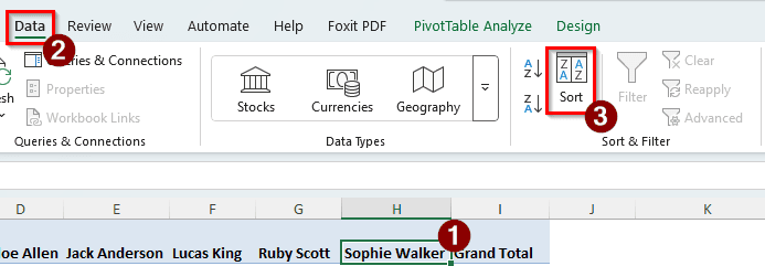
➤ First, click on a cell with the column headings.
➤ Go to the Data tab of the ribbon at the top, and in the Sort & Filter section, click on Sort.
➤ You can do the same thing by clicking on the dropdown arrow of the Column Labels and hitting More Sort Options.
➤ In the new window, there will be three radio buttons. The first radio button, called Manual, will be selected at this point.
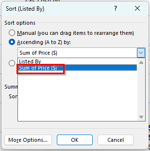
➤ If we select “Ascending (A to Z) by” or “Descending (Z to A) by”, we can further customize the sorting. Let’s select ascending.
➤ There are two options in the dropdown menu of “Ascending (A to Z) by”. The first option is Listed By, which includes the realtor’s names. The second one is the Sum of Price ($). Selecting this will make Excel sort the columns by the price of the properties. We can click OK when we are done, but we aren’t done yet.
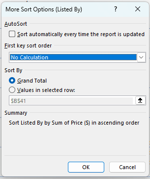
➤ We can access more sorting options by going to More Options.
➤ In the new window, we can disable AutoSort by unchecking the first box. If we do that, we can change the sort order as well.
➤ We can change the Sort By to Grand Total, which is the default. If we change this and set it to Values in selected row, we can custom sort it using selected cells. Click OK to confirm.
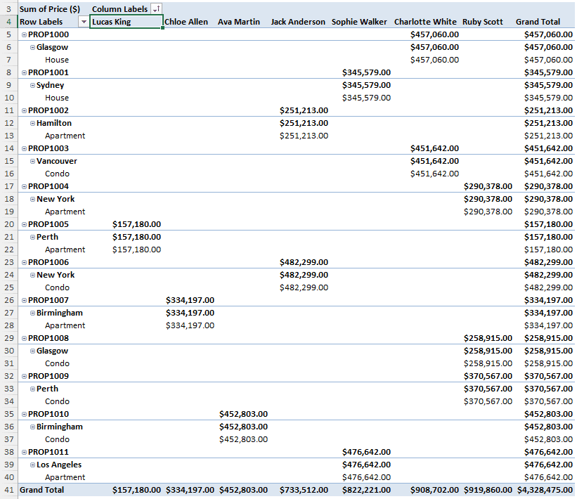
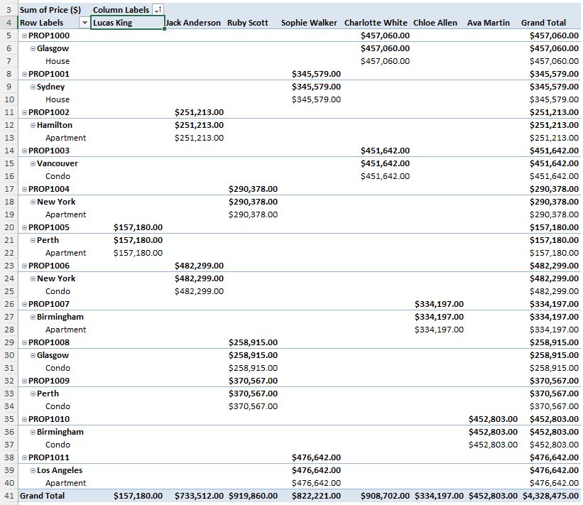
➤ Here is how the pivot table looks after sorting according to the “Sum of Price ($)”.
Defining Custom Lists for Sorting
If you define a custom list for sorting, you can use that for any tables in Excel, not just this particular pivot table. Follow the instructions below to do it:
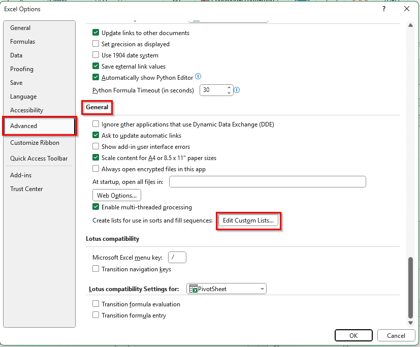
➤ Go to File > Options to open Excel Options.
➤ Go to the Advanced tab, and find the General section on the right. Click on Edit Custom Lists.
➤ There are two methods to create a custom list. You can either add the list entries on the right and click Add, or Import from the Excel sheet using a sorting order you have defined before. We are adding a custom list for the names here and clicking Add to make a list. Afterwards, we click OK to confirm.
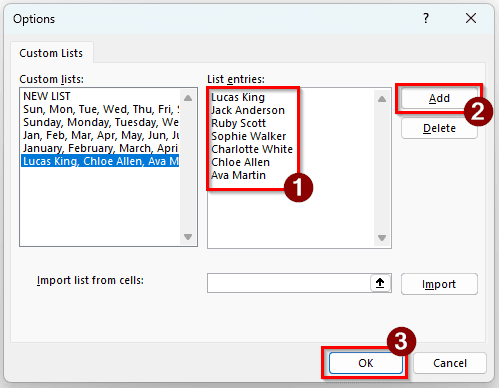
➤ You don’t need to do anything else to apply the custom list. If the entries match the data of your pivot table, Excel will automatically use the custom list to sort.
Frequently Asked Questions
How do I change the order of things in a PivotTable?
In the PivotTable Fields panel on the right, you can drag to move different fields in the Filters, Columns, Rows, and Values sections and change the order of things.
Why is my PivotTable not sorting dates correctly?
There could be several reasons for that. Sorting in pivot tables already works very differently from the regular tables, as the fields are sorted for each category. However, for the dates, a possible reason can be that the dates are not in date format. Excel, by default, stores dates using a numerical format, which makes it easier for it to distinguish and sort. But if the date is stored in text format or something else, it won’t be sorted in the pivot table correctly.
Why is Excel not sorting alphabetically correctly?
Possibilities are that there are characters in the column labels that are obscure or hidden. Those characters can mess up the regular sorting method and cause Excel to make errors.
How to remove sorting in a pivot table?
Right-click on a cell of the pivot table that you want to remove sorting from. From the context menu, go to Sort > More Sort Options. Select the radio button called Manual from the top and hit OK.
Why is the sort greyed out in the Excel PivotTable?
There could be several reasons for this. The file you have opened in Excel might not be writable, especially if it’s downloaded from the internet. You might not have clicked on a cell of the pivot table to activate the sorting options. The data sources used to make the pivot table might not be available at the moment, which might also cause the sorting options to be greyed out.
Wrapping Up
In this article, we have learned different methods to sort columns in pivot tables. Assuming you have read the article carefully, you are able to sort columns in the pivot table properly now. Download the Excel file we have used in this article to try the methods yourself. Leave your questions and feedback below, and stay tuned for more Excel tutorials.