Excel’s MATCH function looks for a specific item in a row or column and tells you its position. While INDEX returns the value at a specific position in a range, INDIRECT converts text into a cell reference that Excel can use.
Combining these functions allows you to look up static and dynamic ranges for specific values. It’s useful for dynamic lookups without rewriting the formula every time. Moreover, these functions work across sheets and workbooks.
To find data from a specific sheet using the INDIRECT, INDEX, and MATCH functions, follow these steps:
➤ Put the sheet name in cell A13 and the lookup value in B13. In the lookup sheet, the data range is A1:D10 where C2:C10 contains the lookup value and we want to pull the corresponding data for that value from the range D2:D10.
➤ For this, insert the following formula:
=INDEX(INDIRECT(“‘” & $A$13 & “‘!D2:D10”), MATCH($B$13, INDIRECT(“‘” & $A$13 & “‘!C2:C10”), 0))
➤ Replace the cell references and ranges according to your dataset. Press Enter.

Apart from such single-match lookups, this article covers other ways of combining the three functions for multi condition lookups, extracting data with calculations, finding values across sheets, matching from an Excel table, etc.
Basic Data Extraction with the INDIRECT, INDEX, and MATCH Functions
In our sample dataset, we have the sales data for the month of January. Therefore, the sheet name is January which contains columns for product codes (Column A), sales agents (Column B), product names (Column C), and prices (Column D).
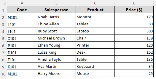
Our goal is to look for a product code from Column A and extract its price from Column D. We can also look up a product directly using the three functions. Here’s how:
Extract Price Based on Product Code Using Cell Reference
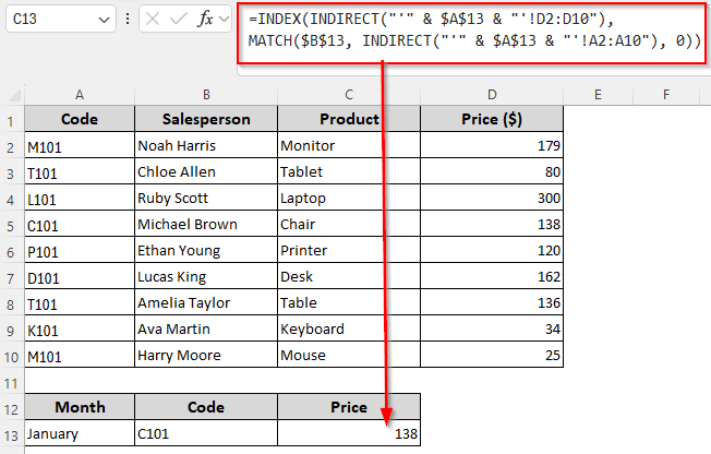
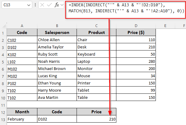
➤ Enter the sheet name in cell A13 and the product code in B13. To return the extracted price for that product code in cell C13, insert this formula in C13:
=INDEX(INDIRECT("'" & $A$13 & "'!D2:D10"), MATCH($B$13, INDIRECT("'" & $A$13 & "'!A2:A10"), 0))
➤ Here, A2:A10 is our lookup range containing the codes and D2:D10 is the result range with the prices. Change the ranges and cell references according to your dataset.
➤ Press Enter.
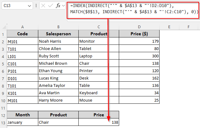
Extract Price Based on Product Name Using Cell Reference
➤ To extract data based on the product name instead of the product code, insert the product name in B13. Enter this formula in C13:
=INDEX(INDIRECT("'" & $A$13 & "'!D2:D10"), MATCH($B$13, INDIRECT("'" & $A$13 & "'!C2:C10"), 0))
➤ Replace the lookup range C2:C10 containing the product names and result range D2:D10 as needed.
➤ Click Enter.
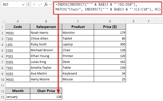
Extract Price Based on Product Name in Text Form
➤ If you want to look for the value Chair in C2:C10 without inserting it in a separate cell, use this formula:
=INDEX(INDIRECT("'" & $A$13 & "'!D2:D10"), MATCH("Chair", INDIRECT("'" & $A$13 & "'!C2:C10"), 0))
➤ Change the cell references and ranges as required.
➤ Press Enter.
Note:
As we’re using the INDIRECT function to reference a sheet, you can change the sheet name in the cell without changing the formula every time.
Using INDIRECT, INDEX, and MATCH for Extracting Data and Calculations
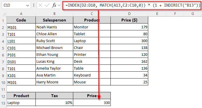
Apart from referencing a sheet, INDIRECT is used to turn texts into cell references. So, we can combine it with INDEX and MATCH for basic calculations with the values in the referencing cells. For example, in our dataset, we can extract the price and add 10% tax or 10% discount to it in the following way:
➤ Insert the product name in cell A13 and the tax or discount rate in cell B13. To calculate the final estimated price after the calculation in cell C13, enter any of the following formulas:
To Calculate Price with 10% Tax
=INDEX(D2:D10, MATCH(A13,C2:C10,0)) * (1 + INDIRECT("B13"))
➤ Replace the lookup range C2:C10, return range D2:D10 and cell references A13 and B13 according to your dataset.
➤ Press Enter.
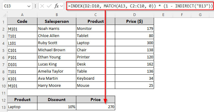
To Calculate Price with a 10% Discount
=INDEX(D2:D10, MATCH(A13, C2:C10, 0)) * (1 - INDIRECT("B13"))
➤ If required, change the cell references and ranges to match your worksheet data.
➤ Click Enter.
Find Values Based on Multiple Conditions
Here, we’ll store our lookup range in another cell and the INDIRECT function will dynamically turn that text string into a reference. After that, we can use the range to look for specific values and return another value from a corresponding cell in a separate column.
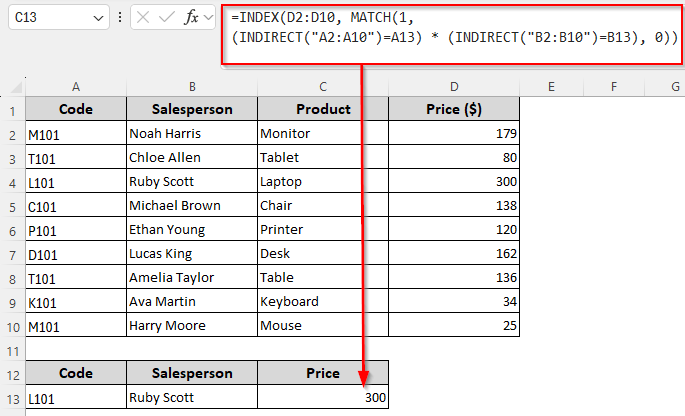
Our goal is to find the price when both Product Code (condition 1) and Salesperson (condition 2) match. Below are the details:
➤ To set the first condition, insert the product code in cell A13 and the salesperson’s name in B13. In cell C13, enter the following formula to return the price:
=INDEX(D2:D10, MATCH(1, (INDIRECT("A2:A10")=A13) * (INDIRECT("B2:B10")=B13), 0))
➤ Replace the result range D2:D10 and lookup ranges A2:A10 and C2:C10 according to your dataset.
➤ Click Enter for Excel 365/2021. For older versions, press Ctrl + Shift + Enter .
Combining INDIRECT, INDEX, and MATCH for Cross-Sheet Lookups
In this method, we’ll create a new sheet named February for the month’s sales data. Similar to the January sheet, this also has product codes in Column A, salesperson names in Column B, product names in Column C, and prices in Column D. We want to pull data from this sheet based on specific criteria.
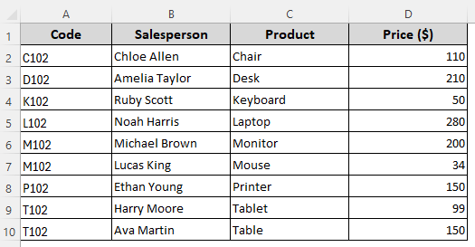
For cross-sheet lookups, we’ll use the INDIRECT function to create a dynamic sheet reference. The INDEX and MATCH functions will then look up for a specific value in that sheet and return the corresponding value from a specified column. Let’s get to the steps:
Lookup Using Cell References
➤ Put the sheet name in cell A13 and the lookup value in B13. To get the corresponding price from Column D (D2:10), insert this formula:
=INDEX(INDIRECT("'" & A13 & "'!D2:D10"), MATCH(B13, INDIRECT("'" & A13 & "'!A2:A10"), 0))
➤ Change the lookup range A2:A10 and result range D2:D10 as per your dataset.
➤ Click Enter.
Lookup Using Direct Values (Texts)
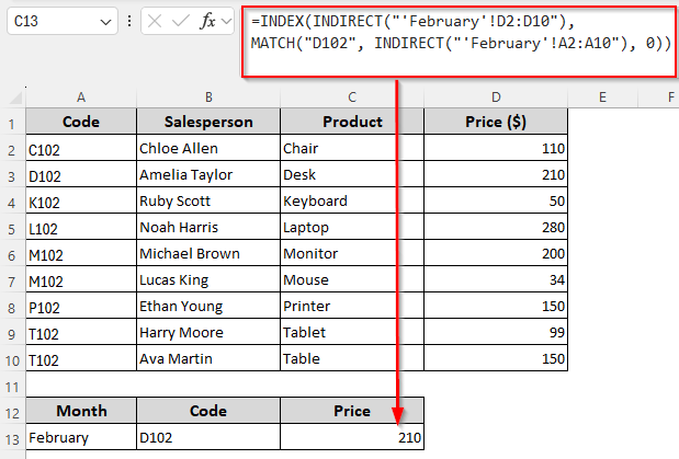
➤ To look for the code D102 and return the price for the product matching the code in the February sheet, use this formula:
=INDEX(INDIRECT("'February'!D2:D10"), MATCH("D102", INDIRECT("'February'!A2:A10"), 0))
➤ Replace the sheet name February, lookup value D102, and ranges as required.
➤ Press Enter.
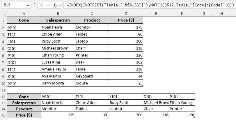
Using the INDIRECT, INDEX, and MATCH Functions to Match Values Across Tables
Our new table has rows for product codes, salesperson names, product names, and prices. In the first column, we have 5 product codes.
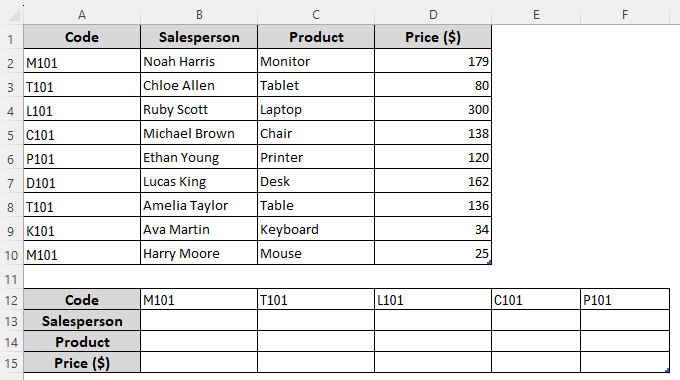
We’ll complete the table by pulling data from the first table matching our search criteria. Here’s how:
➤ To get the salesperson’s name who sold the product for the code M101, we’ll enter the following formula in the first intersection of Salesperson and M101 (cell B13):
=INDEX(INDIRECT("Table1["&$A13&"]"),MATCH(B$12,Table1[[Code]:[Code]],0))
➤ Here, $A13 is the cell containing the lookup column heading, B$12 contains the second lookup value which is in the column Code. Change the references and values according to your dataset.
➤ Press Enter to extract the name from the first column.
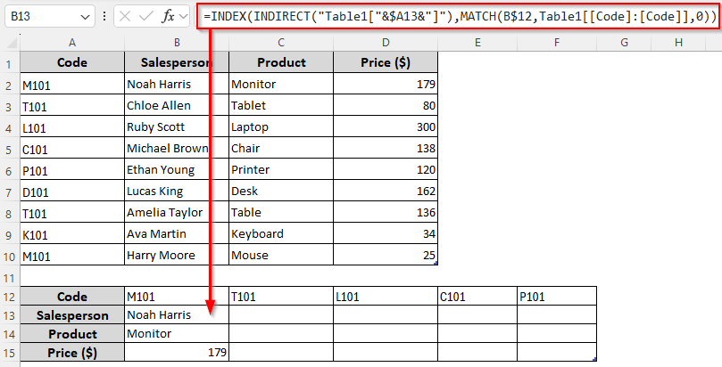
➤ Use the fill handle (+ sign on the bottom corner of the cell) to drag the formula down first and then across the columns to fill the remaining cells.
Frequently Asked Questions
How to avoid errors with INDIRECT, INDEX, and MATCH functions?
To avoid errors and replace them with blanks, you need to wrap your formula in IFERROR.
For example, here’s how to combine IFERROR with a basic lookup formula with INDIRECT, INDEX, and MATCH:
=IFERROR(INDEX(INDIRECT(“‘” & $A$13 & “‘!D2:D10”), MATCH($B$13, INDIRECT(“‘” & $A$13 & “‘!C2:C10”), 0)), “”)
What is the difference between the INDEX and MATCH functions in Excel?
The INDEX function returns the value at a specific row and column in a range. For example, if cell A1 contains 50, you can use the following formula to return 50 in any cell:
=INDEX(A1)
On the other hand, MATCH returns the position (row or column number) of a value in a range. For instance, if our data range is B1:B10 and we have the value Math in cell B2, the following formula returns 2:
=MATCH(“Math”, B1:B10, 0)
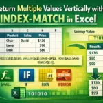
Can INDIRECT, INDEX, and Match return multiple values?
No, combining the INDIRECT, INDEX, and MATCH functions will give you only a single value (the first match found). That’s because INDEX/MATCH can return only one cell unless wrapped in other array-friendly formulas. You can use the FILTER or TEXTJOIN functions to get multiple values for a lookup.
Concluding Words
While the basic functions of INDIRECT, INDEX, and MATCH remain the same, you can use them in many different ways to extract data or find a match across sheets. They also allow for complex calculations using dynamic ranges.
Although the INDEX and MATCH functions are enough for a basic lookup, nesting the INDIRECT function gives you more flexibility and allows you to change values and references without editing the actual formula.