
Most Excel users are comfortable adding up the numbers across a single column. Drag cells or do a quick SUM and you’re done. But things get trickier when your data extends to several columns, like sales split to months, expenses divided by departments, and performance scale spread across categories. And, with just SUM, you are left with no option but to juggle with formulas, helper columns, and not-so-helpful methods. The result is error-prone data. That’s where the SUMPRODUCT can help you. It is not just any mere sum formula. Rather, it allows you to calculate values across various columns based on applied conditions.
To use SUMPRODUCT across multiple columns in Excel, you can use the following steps-
➤ Identify the columns that you want to add together.
➤ Determine their ranges.
➤ Select a cell to display its output. Give it a proper header.
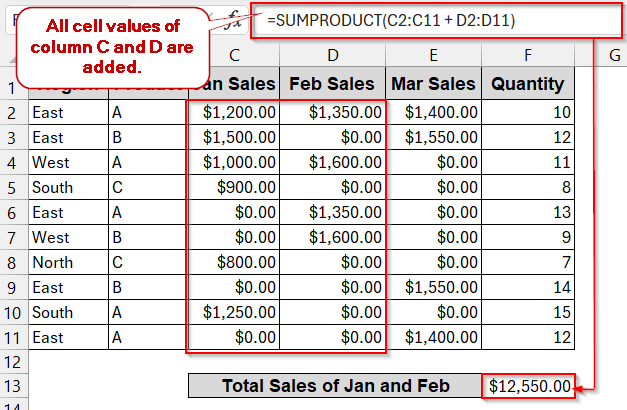
➤ In the cell, write the SUMPRODUCT formula – =SUMPRODUCT(C2:C11 + D2:D11),
Here, the first 10 columns C and D cells are added, excluding the header.
➤ Press Enter to display the output.
With the easy sum of the columns, SUMPRODUCT can sum up the entire range of cells filtered under various conditions. To tackle real-world dataset problems, AND/OR logic can also fine-tune the calculation per your requirement. And, of course, there are more dynamic and automated solutions like VBA Macros that can speed up the process. Don’t worry, we have it all covered. By the end of this guide, you’ll see how SUMPRODUCT can be used in multiple ways and multiple scenarios.
SUMPRODUCT Across Columns Without Conditions
In simple reports, where it is necessary to calculate the sum across two or more columns, you can rely on SUMPRODUCT. It is beginner-friendly and also allows you to sum without any specific criteria or logic.
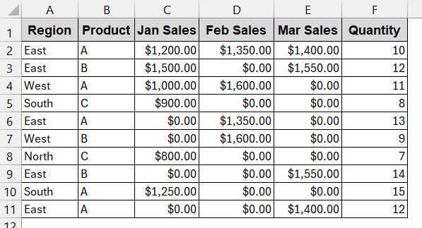
From the above dataset, you will find the total sales of January and February.
Steps:
➤ At first, understand which columns need to be included. For this example, we need column C (Jan Sales) and D (Feb Sales).
➤ Identify their ranges.
➤ Select a new cell to display the result. Give it a proper header (e.g, Total Sales of Jan and Feb).
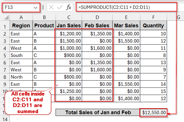
➤ Write the basic SUMPRODUCT formula –
=SUMPRODUCT(C2:C11 + D2:D11)
Here, C2:C11 and D2:D11 are the cell ranges of Jan and Feb sales.
➤ Press Enter to display the output in the selected cell.
Notes:
➨ All the ranges must be the same for the SUMPRODUCT to produce a result.
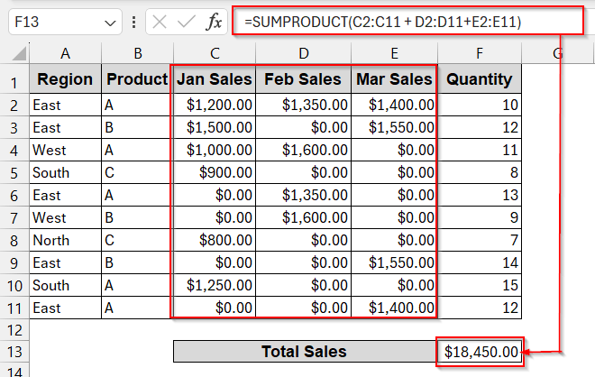
➨ To extend this to more columns, just add column ranges one after another inside the formula-
=SUMPRODUCT(C2:C11 + D2:D11 + E2:E11)
Using SUMPRODUCT Across Multiple Columns with Criteria
In practical datasets, you hardly need to just sum your columns. Usually, we need to sum the cells across multiple columns using various criteria. As a result, it filters some cells that satisfy our requirement and only includes them in the formula. This is the best part of the SUMPRODUCT, as it helps to complete the process without complex formulas or helper columns.
Here, we will find the total sales for all the months from the ‘West’ region.
Steps:
➤ Identify what columns you need to sum (e.g, C, D, and E).
➤ Locate which column has the criteria based on which you want to filter the cells of the required column. In this case, the Region column (A) has the criteria ‘West’, which is the criteria here.
➤ Ensure the range of cells of each column is the same.
➤ Select a cell to display the output.
➤ Write the formula of SUMPRODUCT with criteria –
=SUMPRODUCT(($A$2:$A$11="West") * ($C$2:$C$11 + $D$2:$D$11 + $E$2:$E$11))
Here, the ($A$2:$A$11=”West“) ensures the ‘West’ is selected for column A to filter the ranges of $C$2:$C$11, $D$2:$D$11, and $E$2:$E$11.
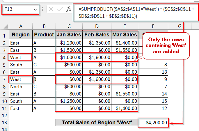
➤ Press Enter to get the output.
Notes:
➨ You can replace the text ‘West’ with the cell reference. Cells A4 and A7 contain ‘West’; you can use either of them in the formula instead of text. This will make the data more dynamic.
➨ To add more criteria, you can simply add them one after another before summing.
=SUMPRODUCT(($A$2:$A$11=”West”)*($B$2:$B$11=”A”)*($C$2:$C$11+$D$2:$D$11+$E$2:$E$11)),
here, $B$2:$B$11=”A” is another criteria. This ensures it only sums the rows of C, D, and E that have both the Region ‘West’ and the Product ‘A’ in them.
Apply OR Logic in SUMPRODUCT for Multiple Columns in Excel
OR logic is so common in conditionals, but it is hardly supported in sum formulas. For example, if you want to calculate the result, even if one of the conditions satisy, there is no way other than an OR logic. Luckily, SUMPRODUCT has the functionality of combining any logic.
Here, we will find the total sales of the products from the ‘West’ or ‘South’ regions.
Steps:
➤ Start by finding the resultant columns that need to be added (e.g, – C, D, and E).
➤ Identify the columns that contain the criteria. Here, it is column A (Region).
➤ Select a cell to display the output. Give it a proper header.
➤ Write the SUMPRODUCT formula –
=SUMPRODUCT((($A$2:$A$11="West") + ($A$2:$A$11="South")) * ($C$2:$C$11 + $D$2:$D$11 + $E$2:$E$11)),
Here $A$2:$A$11=”West” and $A$2:$A$11=”South” are two criteria, ‘West’ and ‘South’. They are separated by ‘+,’ which indicates OR logic.
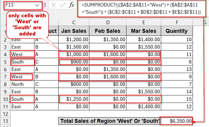
➤ Press Enter to get the output in the selected cell.
Notes:
For multiple criteria with OR logic in different columns, you can use the same syntax and logic. But, remember to wrap the OR logic in –(…>0). It ensures that when both conditions are satisfied in the same row, it does not get calculated twice.
=SUMPRODUCT(–((($A$2:$A$11=”West”) + ($B$2:$B$11=”A”))>0) * ($C$2:$C$11+$D$2:$D$11+$E$2:$E$11))
Dynamic Cell Selection in SUMPRODUCT with INDEX Function
You have seen from the previous methods that you have hardcoded the column ranges and the text of the criteria. But it’s not that flexible, especially when you have tons of data to work with. In that case, you can select cells dynamically if you do a simple addition to your basic formula – INDEX.
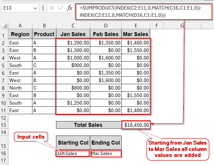
For example, let’s assume you need to find the total sales of all three months. That means we have three columns to work with and have no criteria.
Steps:
➤ For dynamic cell selection, you need to prepare input cells. Choose two cells for the and write the start and end column (e.g, Jan Sales and Mar Sales).

➤Identify your column headers that match the input and the column references.
➤ Ensure the columns match, use the MATCH formula –
=MATCH(C16, C1:E1, 0)
Where C16 is the input cell of the starting column, and C1:E1 is the total range of the columns selected.
➤ This will return the column number. It will return 1 for the starting column and 3 for the ending column for this example.
➤ If your MATCH function works properly, use the INDEX function, combining with MATCH and SUMPRODUCT.
=SUMPRODUCT(INDEX(C2:E11,0,MATCH(G1,C1:E1,0)):INDEX(C2:E11,0,MATCH(H1,C1:E1,0)))
where INDEX(C2:E11,0,MATCH(G1,C1:E1,0)) points to the first column and INDEX(C2:E11,0,MATCH(H1,C1:E1,0)) points to the second column.
➤ Press Enter to display the output.
Notes:
This method can also be combined with the criteria mentioned above. It works best when you need to calculate across a large set of columns.
Create a VBA UDF for Multi-Column SUMPRODUCT
Another dynamic way to transform your SUMPRODUCT is the VBA Macros. Whether you want to do a simple sum, combine multiple criteria, or use OR/AND logic, you can create a custom VBA User Defined Function (UDF). This will help you work with the complex formula easily and get faster results.
In this method, you will find the total sales from January to March, having the product in the region ‘West’.
Steps:
➤ Identify the columns and ranges that need to be included in the formula.
➤ Go to the Developers tab and click on Visual Basic.

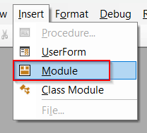
➤ In the VBA editor, click on Insert -> Module.
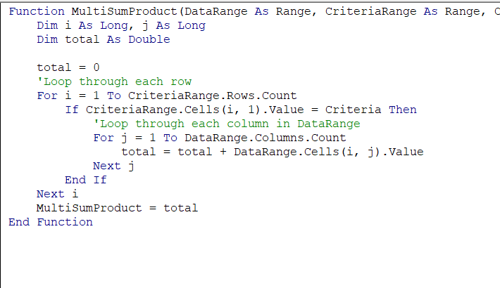
➤In the new module, paste the code below –
Function MultiSumProduct(DataRange As Range, CriteriaRange As Range, Criteria As String) As Double
    Dim i As Long, j As Long
    Dim total As Double
    total = 0
    'Loop through each row
    For i = 1 To CriteriaRange.Rows.Count
        If CriteriaRange.Cells(i, 1).Value = Criteria Then
            'Loop through each column in DataRange
            For j = 1 To DataRange.Columns.Count
                total = total + DataRange.Cells(i, j).Value
            Next j
        End If
    Next i
    MultiSumProduct = total
End Function
➤ Save the code snippet by Ctrl + S and close the window.
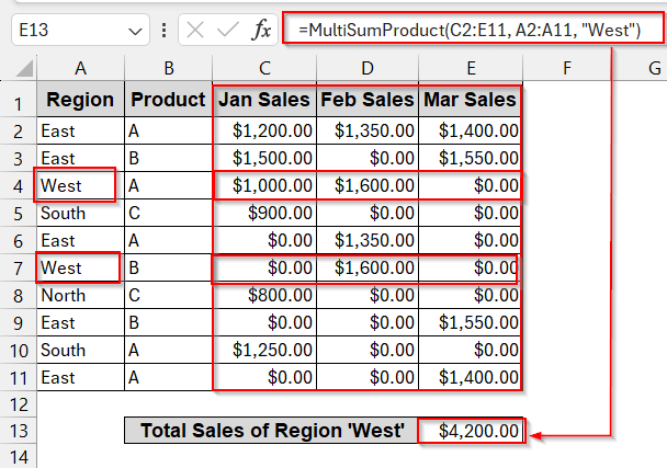
➤ Select a cell to display the output. Give it a proper header.
➤ Use the newly created formula of MultiSumProduct–
=MultiSumProduct(C2:E11, A2:A11, "West")
Here, the selected column range is given before the criteria. The criteria range and the criteria text (or reference) follow after that.
➤ Press Enter to display the result.
Notes:
This VBA function can work with extended columns and criteria.
Frequently Asked Questions
Can SUMPRODUCT add values across multiple columns at once?
You can add values across multiple columns by SUMPRODUCT. You need to give a ‘+’ sign and put the range of columns one after another. The ranges of the SUMPRODUCT must be the same.
How do I apply OR logic when summing across multiple columns?
To apply the OR logic when summing across columns, you need to add the criteria in the beginning and separate them by ‘+’ signs.
=SUMPRODUCT(($A$2:$A$11=”East”)+ ($A$2:$A$11=”West”) * (C2:C11+D2:D11+E2:E11))
Why do I get #VALUE when ranges are from different columns?
You might get #VALUE in the SUMPRODUCT due to inconsistent ranges over columns. Ensure your columns all have the same selected ranges inside the SUMPRODUCT.
Which is faster — SUMPRODUCT or SUM across columns?
Though SUM is faster, SUMPRODUCT is better. Unlike SUM, it enables users to calculate across multiple columns based on multiple criteria and logics.
Can I make SUMPRODUCT dynamic to speed up the process?
You can make the SUMPRODUCT dynamic by using cell references or using the INDEX function. Other than that, VBA Macros can be a great alternative for faster and dynamic solutions.
Concluding Words
Mastering SUMPRODUCT in multiple columns is a powerful skill you need while working in Excel. Whether you are adding monthly sales, filtering columns based on conditions, applying various types of logics, or making dynamic user input ranges, SUMPRODUCT does the exact thing. It gives accurate data, keeping your data clean and compact. When you blend all the methods, you get the speed, flexibility, and customizations. Literally, the best of all worlds. With these tools, you can handle any multi-column analysis with ease and confidence.